From Ancient Skies to Kepler’s Laws

2,000 Years of Puzzles,
Three Elegant Rules

Dr. Anna Rosen

February 2, 2026

The planets wander

“The planets wander… sometimes they appeared to move backward.”

For 2,000 years, astronomers asked why.

0–1 min. Set the historical context. “The Greeks called them planetes — wanderers. And they did something that seemed impossible: sometimes they appeared to move backward.”

Credit: cococubed.com

Quick visual grounding: the Solar System layout before the retrograde puzzle.

Today’s Learning Objectives

By the end of today, you can:

• Explain retrograde motion as perspective + geometry
• Describe why models change (evidence + simplicity)
• State Kepler’s three laws
• Use Kepler III to relate \(P\) and \(a\) (ratio or Sun-only form)
• Distinguish empirical patterns from physical mechanisms

1–2 min. Frame the lecture: “Today we trace 2,000 years of astronomy in 50 minutes. The payoff: three laws that describe all planetary motion.”

The Cosmic Puzzle

Why do planets move backward?

Section transition. 30 sec.

The Wanderers

Credit: cococubed.com

Stars rise and set predictably.

But a handful of bright lights wandered among the fixed stars.

Sometimes they appeared to stop, reverse direction, then resume their journey.

2–3 min. “The Greeks called them planetes. Mars was the most dramatic — sometimes it seemed to drift backward for weeks.”

Retrograde Motion — The Puzzle

What could cause a celestial body to move backward?

Spoiler: retrograde is an apparent motion — an illusion of perspective.

Like passing a slower car: it can look like it drifts backward against distant mountains.

3–4 min. Draw the highway analogy on the board. “Your car, their car, distant mountains. As you pass them, what appears to happen?”

The Highway Analogy

• Earth: faster, inner orbit
• Mars: slower, outer orbit
• Stars: distant background

As Earth passes Mars, Mars appears to drift backward against the stars.

But Mars never reverses its orbital direction.

4–5 min. “Earth orbits faster than Mars. When we pass Mars, it appears to drift backward against the distant stars.”

Quick Check: Retrograde Motion

During Mars retrograde, Mars is actually moving:

• Backward in its orbit
• Forward in its orbit
• Stopped in space
• Falling toward the Sun

1 min. Poll. Most common misconception: students think Mars actually reverses.

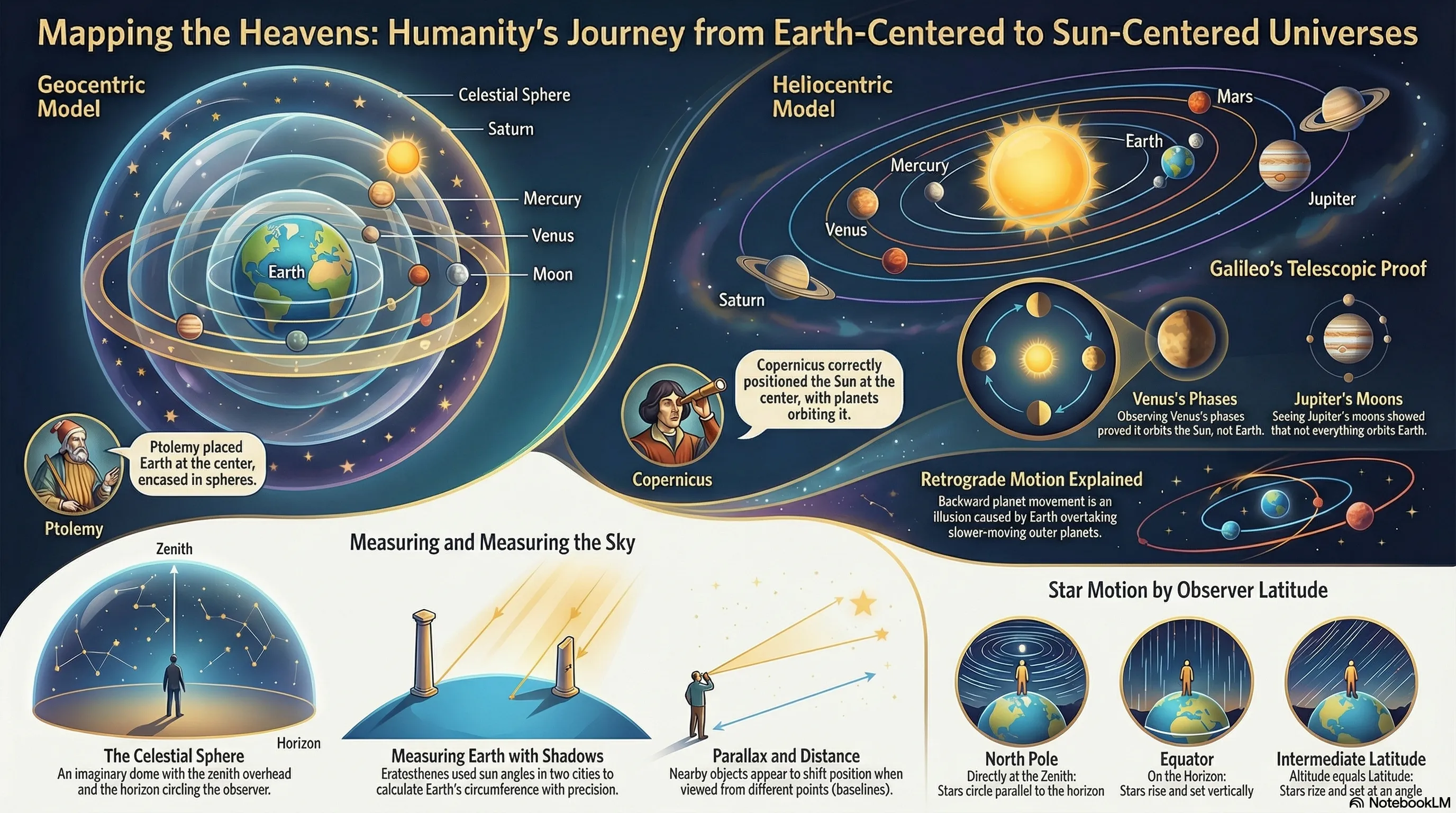
The Ancient Answer

Earth at the center

Ptolemy’s Geocentric Model (~150 CE)

Credit: Illustration: A. Rosen (SVG)

Earth felt obviously central:

• We don’t feel Earth moving
• Stars rotate around us
• It matched everyday experience

5–6 min. “For nearly 1,500 years, this was the accepted model.”

The Epicycle Solution

Ptolemy proposed epicycles:

• Planet moves on a small circle (epicycle)
• Epicycle center moves on a larger circle (deferent)
• Combined motion can trace a loop (apparent retrograde)

Accurate, but complex: by medieval times the model needed dozens of circles.

6–7 min. “Accurate but ugly. A baroque machinery of nested circles.”

Spot the Assumption

The geocentric model protected two assumptions:

1. Earth is stationary and central — we don’t feel motion, so we must not be moving

2. Circular motion is perfect — orbits must be circles because circles are “perfect”

What happens when we challenge these?

7–8 min. “Every scientific revolution involves challenging assumptions that everyone took for granted.”

The Revolution Begins

Copernicus, Galileo, Tycho, Kepler

Copernicus (1543): A Simpler Idea

What if the Sun is at the center?

Geocentric (Ptolemy)

• Earth at center
• Epicycles needed for retrograde
• Dozens of circles

Heliocentric (Copernicus)

• Sun at center
• Retrograde = Earth passing outer planets
• No epicycles needed for retrograde!

8–10 min. “Copernicus’s idea was conceptually simpler. Retrograde was just geometry.”

Quick Check: The Copernican Shift

What was the key advantage of Copernicus’s heliocentric model?

• It was more accurate at predicting planetary positions
• It explained retrograde motion as geometry rather than requiring epicycles
• It was immediately accepted by the Church
• It used ellipses instead of circles

1 min. iClicker poll. Note: Copernicus still used circles, so some complexity remained.

The Evidence Mounts

Galileo (1610) used telescopes to test models:

• Jupiter has moons — not everything orbits Earth
• Venus shows phases — consistent with heliocentrism

Evidence did not end the controversy.

10–12 min. “The scientific evidence eventually won — but it took courage to follow it.” Galileo faced the Inquisition (1633) and spent his remaining years under house arrest.

Tycho Brahe: The Master Observer

20+ years of planetary observations

Greatest naked-eye observer in history

Tycho’s data was unprecedented in precision.

When he died in 1601, his observations passed to his young assistant…

Johannes Kepler

12–13 min. “Tycho collected the data. Kepler would find the pattern hidden within.”

Kepler’s Laws

The Main Event

Section transition. “Now we get to the good stuff. Three laws that describe all planetary motion.”

Kepler’s Struggle

Kepler inherited Tycho’s precision Mars data.

For years he tried circles.

An 8 arcminute mismatch forced a new shape: an ellipse.

Suddenly, the orbit fit.

13–15 min. “Kepler later wrote that he felt like he had ‘awoken from a sleep.’ One ellipse replaced dozens of circles.”

Kepler’s First Law: The Shape of Orbits

Planets orbit the Sun in ellipses, with the Sun at one focus.

Credit: cococubed.com

15–17 min. “Not circles — ellipses. And the Sun isn’t at the center; it’s at one focus.”

What’s an Ellipse?

Credit: (A. Rosen/Codex)

An ellipse has two special points called foci.

Key property: Sum of distances from any point to both foci is constant.

Eccentricity (\(e\)): How “squashed” the ellipse is

• \(e = 0\) means a perfect circle
• \(e\) close to 1 means a very elongated ellipse

17–18 min. “A circle is just a special ellipse with eccentricity zero.”

Key Orbital Terms

Term	Symbol	Definition
Semi-major axis	\(a\)	Half the longest diameter; “average” orbital distance
Eccentricity	\(e\)	How “squashed” (0 = circle, near 1 = elongated)
Perihelion	\(r_p\)	Closest point to Sun; \(r_p = a(1-e)\)
Aphelion	\(r_a\)	Farthest point from Sun; \(r_a = a(1+e)\)

The Sun sits at one focus, not the center.

18–19 min. “These terms will come up again and again. The semi-major axis is the key distance measure.”

Real Planetary Eccentricities

Planet	Eccentricity	Description
Venus	0.007	Nearly circular
Earth	0.017	Nearly circular
Mars	0.093	Noticeably elliptical
Mercury	0.206	Most eccentric planet
Halley’s Comet	0.97	Extremely elongated

Most planets have nearly circular orbits — this is why Ptolemy got reasonably good results with circles.

19–20 min. “The ellipses are subtle for most planets. But subtle isn’t zero.”

Quick Check: Eccentricity

An orbit with eccentricity \(e = 0\) would be:

• A very elongated ellipse
• A perfect circle
• A parabola
• Impossible for a planet

1 min. iClicker poll.

Kepler’s Second Law: Orbital Speed

A line connecting a planet to the Sun sweeps out equal areas in equal times.

Credit: cococubed.com

20–22 min. “This is the law of equal areas. What does it mean for orbital speed?”

What “Equal Areas” Means

Perihelion (close to Sun):

• Smaller \(r\)
• Faster speed

Aphelion (far from Sun):

• Larger \(r\)
• Slower speed

Bottom line: planets speed up when closer to the Sun.

22–23 min. “Think of cutting wedges out of paper. Near perihelion: short and fat. Near aphelion: long and thin. Same area.”

Credit: cococubed.com

Reinforce why closer = faster through angular momentum conservation.

The Ice Skater Analogy

Think of an ice skater spinning with arms extended.

Arms in: spins faster

Arms out: spins slower

This is conservation of angular momentum.

Same idea: closer to the Sun means faster; farther means slower.

23–24 min. “Kepler described the pattern; Newton would later explain why.”

Real Example: Earth’s Orbit

Position	Date	Distance from Sun	Earth’s Speed
Perihelion	~Jan 3	147.1 million km	30.3 km/s
Aphelion	~Jul 4	152.1 million km	29.3 km/s

Earth’s Orbit: What This Means

• Earth moves about 3% faster near perihelion than near aphelion.
• Northern Hemisphere winter is slightly shorter than summer.

24–25 min. “A subtle effect, but real and measurable.”

Quick Check: Fastest Point

A planet is moving fastest when it is at:

• Aphelion (farthest from the Sun)
• Perihelion (closest to the Sun)
• Halfway between perihelion and aphelion
• The planet moves at constant speed

1 min. iClicker poll.

Predict First!

Before we see the law: if we double the orbital size (\(a \to 2a\)), the orbital period \(P\) becomes:

1. \(2\times\)

2. \(\approx 2.8\times\)

3. \(4\times\)

4. \(8\times\)

30 s. Have students commit to an option. Then reveal: from \(P^2 \propto a^3\), doubling \(a\) multiplies \(P\) by \(\sqrt{2^3}=\sqrt{8}\approx 2.8\).

Kepler’s Third Law: The Period-Distance Relation

The square of a planet’s orbital period is proportional to the cube of its semi-major axis.

\[P^2 \propto a^3\]

25–27 min. “This is the harmonic law. It connects distance and time.”

Reading Kepler III

Let’s unpack the symbols:

• \(P\): orbital period (time per orbit)
• \(a\): semi-major axis (a measure of orbit size)

In plain English: if you increase orbit size, the period increases more than linearly.

Why Outer Planets Take Longer

Two effects compound:

1. They have farther to travel (larger orbit circumference)

2. They move slower (farther from the Sun means weaker gravitational pull)

These combine to give the precise \(P^2 \propto a^3\) relationship.

27–28 min. “It’s not just that Jupiter is farther — it’s also moving slower.”

How to Use Kepler’s Third Law

Form 1: Ratio Method (recommended default)

\[\left(\frac{P_2}{P_1}\right)^2 = \left(\frac{a_2}{a_1}\right)^3\]

Compare two objects orbiting the same central body.

Form 2: Sun-only Scaling

For objects orbiting the Sun, with \(P\) in years and \(a\) in AU:

\[\left(\frac{P}{1\,\text{yr}}\right)^2 = \left(\frac{a}{1\,\text{AU}}\right)^3\]

28–29 min. “The ratio method is safest — no unit confusion. The Sun-only form is a convenient shortcut.”

Worked Example 1

Problem: A planet orbits the Sun at \(a = 4\) AU. What’s its period?

\[\left(\frac{P}{1\,\text{yr}}\right)^2 = \left(\frac{4\,\text{AU}}{1\,\text{AU}}\right)^3 = 64\]

\[P = \sqrt{64} \times 1\,\text{yr} = \boxed{8 \text{ years}}\]

29–30 min. Walk through step by step.

Worked Example 2

Problem: A comet has orbital period \(P = 27\) years. What’s its semi-major axis?

\[\left(\frac{27\,\text{yr}}{1\,\text{yr}}\right)^2 = \left(\frac{a}{1\,\text{AU}}\right)^3\]

\[729 = \left(\frac{a}{1\,\text{AU}}\right)^3\]

\[a = \sqrt[3]{729} \times 1\,\text{AU} = \boxed{9 \text{ AU}}\]

30–31 min. “Cube root of 729 is 9, because \(9\times 9\times 9 = 729\).”

Quick Check: Basic Calculation

An asteroid orbits the Sun at a distance of 4 AU. What is its orbital period?

• 4 years
• 8 years
• 16 years
• 64 years

1 min. iClicker poll. Same as worked example — reinforcement.

Solar System Examples

Planet	\(a\) (AU)	\(a^3\)	\(P\) (years)	\(P^2\)
Earth	1.00	1.00	1.00	1.00
Mars	1.52	3.51	1.88	3.53

Notice: \(a^3 \approx P^2\).

31–32 min. “Kepler’s Third Law fits perfectly across the entire Solar System.”

Solar System Examples (continued)

Planet	\(a\) (AU)	\(a^3\)	\(P\) (years)	\(P^2\)
Jupiter	5.20	141	11.86	141
Saturn	9.54	868	29.46	868

Same pattern: \(a^3 \approx P^2\).

Quick Check: Scaling

If a planet’s orbital distance \(a\) increases by a factor of 4, its orbital period \(P\) increases by a factor of:

• 4
• 8
• 16
• 64

1–2 min. Poll, then explain. Reasoning: from \(P^2 \propto a^3\), we get \(P \propto a^{3/2}\). If \(a\) increases by 4, then \(P\) increases by \(4^{3/2} = 8\).

The Limits of Patterns

What Kepler could — and couldn’t — explain

What Kepler Could Do

• Predict planetary positions for centuries
• Calculate eclipses and conjunctions
• Replace dozens of epicycles with three elegant laws

For the first time, humanity had a precise mathematical description of planetary motion.

32–34 min. “This was a triumph of pattern recognition.”

What Kepler Couldn’t Explain

1. Why ellipses? Why not circles?

2. Why do planets speed up when closer?

3. Why \(P^2 \propto a^3\)?

4. Does it work around other stars?

34–35 min. “Patterns aren’t explanations. Kepler could tell you that, but not why.”

Empirical vs. Physical Laws

Empirical law: A pattern from data. Describes what happens.

Physical law: Explains why it happens.

Kepler’s laws are empirical.

They describe what planets do, beautifully and precisely.

But they don’t explain the underlying mechanism.

35–36 min. “The distinction matters. Empirical laws can’t predict what happens in new situations.”

Quick Check: Empirical vs. Physical

Kepler’s laws are considered “empirical” rather than “physical” because:

• They are approximately true, not exactly true
• They describe patterns without explaining the underlying mechanism
• They only apply to the Solar System
• They were discovered before telescopes existed

1 min. Poll.

The Setup for Newton

Newton (1687) gives the mechanism:

\[F = \frac{Gm_1m_2}{r^2}\]

Symbols:

• \(F\): force magnitude (N)
• \(m_1, m_2\): masses (kg)
• \(r\): separation between centers (m)

Key idea: \(F \propto 1/r^2\).

Assumptions (for this course): Newtonian gravity, two-body approximation, and objects behave like point masses / spherical bodies.

36–38 min. “Kepler gave us a rulebook. Newton will give us the reason the rulebook exists.” Assumptions to model explicitly (briefly): Newtonian gravity; objects behave like point masses / spherically symmetric bodies; two-body approximation.

How Science Evolves

From epicycles to ellipses

The Power of Simplicity

Era	Model	Complexity
Ptolemy (~150 CE)	Geocentric + epicycles	Dozens of circles
Copernicus (1543)	Heliocentric + circles	Fewer circles, still complex
Kepler (1609-1619)	Heliocentric + ellipses	3 laws, no epicycles

Each step toward truth was also a step toward simplicity.

38–40 min. “Occam’s Razor vindicated. When you’re adding complexity upon complexity, question your assumptions.”

The Chain of Discovery

• Islamic scholars preserved Greek astronomy
• Copernicus proposed heliocentrism
• Tycho gathered precision data
• Kepler found the patterns
• Newton explained the physics

40–42 min. “And it continues. Newton’s laws would eventually be refined by Einstein.” Emphasize: science is a community effort across cultures and centuries.

Credit: (A. Rosen/NotebookLM)

42–43 min. Let the infographic speak. “2,000 years of progress in one image.”

Key Takeaways

1. Retrograde is apparent (a geometry effect).

2. Kepler I: ellipses, Sun at a focus.

3. Kepler II: equal areas in equal times.

43–45 min. Recap the main points.

Key Takeaways (continued)

4. Kepler III: \(P^2 \propto a^3\) (use ratio or Sun-only form).

5. Kepler describes patterns; Newton explains mechanisms.

6. Better models are often simpler and more predictive.

Coming Up: Newton’s Gravity

Next lecture: Newton transforms patterns into physics.

We’ll see how one equation explains Kepler’s three laws.

Reading: Lecture 6 Reading Companion

Demo: Kepler’s Laws (Newton Mode): ../../../demos/keplers-laws/

45–50 min. Preview next lecture and remind about reading/demo.

Questions?

Kepler gave us the patterns.

Newton will give us the physics.

Remaining time for questions (before optional math appendices).

Numerical Verification

Checking our work with real data

Optional section for students who want to see the math verified explicitly.

Verifying Kepler III: Mars

Given data:

• Mars semi-major axis: \(a = 1.524\) AU
• Mars orbital period: \(P = 687\) days

Step 1: Convert period to years

\[P = 687 \text{ days} \times \frac{1 \text{ year}}{365.25 \text{ days}} = 1.881 \text{ years}\]

Step 2: Check \(P^2 = a^3\)

\[P^2 = (1.881)^2 = 3.538 \text{ yr}^2\]

\[a^3 = (1.524)^3 = 3.540 \text{ AU}^3\]

Match within rounding: \(3.538 \approx 3.540\) (0.06% difference from rounding)

Walk through unit conversions explicitly. “Notice the units: yr\(^2\) on the left, AU\(^3\) on the right. They match because we defined our system so that Earth has \(P=1\) yr at \(a=1\) AU.”

Unit Analysis: Why \(\mathrm{yr}^2 = \mathrm{AU}^3\)?

Why does the shortcut look like time-squared equals distance-cubed?

The full physics statement is:

\[P^2 = \left(\frac{4\pi^2}{GM_\odot}\right) a^3\]

The constant \(\frac{4\pi^2}{GM_\odot}\) is doing the unit conversion.

Unit Analysis: What the Constant Means

• Sun-only shorthand: \(a\) in AU and \(P\) in years \(\Rightarrow P^2 \approx a^3\)
• Change units or change the central mass \(\Rightarrow\) use the full form (or the ratio method)

“This is why I emphasize units so much. The simple formula is a gift of choosing good units.”

Unit Analysis: Why the Ratio Method Is Safe

• Compare two orbits around the same central mass: hidden constants cancel.
• It reduces unit mistakes and keeps the physics visible.

Verifying Kepler III: Jupiter

Given data:

• Jupiter semi-major axis: \(a = 5.203\) AU
• Jupiter orbital period: \(P = 4333\) days

Convert and verify:

\[P = 4333 \text{ days} \times \frac{1 \text{ yr}}{365.25 \text{ days}} = 11.86 \text{ yr}\]

\[P^2 = (11.86)^2 = 140.7 \text{ yr}^2\]

\[a^3 = (5.203)^3 = 140.9 \text{ AU}^3\]

Match within rounding: \(140.7 \approx 140.9\)

“Same pattern. Kepler’s law works across the entire Solar System.”

Common Unit Mistake: Mixing Units

Mistake (unit mismatch):

“\(a = 778\) million km, \(P = 12\) years, so \(P^2 = 144\) and \(a^3 = 4.7 \times 10^{26}\)… they don’t match!”

Fix (convert first):

\[a = 778 \times 10^6 \text{ km} \times \frac{1 \text{ AU}}{1.496 \times 10^8 \text{ km}} = 5.20 \text{ AU}\]

Then compare \(P^2\) (in yr\(^2\)) to \(a^3\) (in AU\(^3\)).

Common Unit Mistake: Forgetting Squares and Cubes

Mistake (wrong powers):

“\(P = 12\) years and \(a = 5.2\) AU, so \(12 = 5.2\)… wrong!”

Fix: Kepler III is about \(P^2\) and \(a^3\).

In Sun-only units (years and AU), you can do a quick consistency check:

\[(12)^2 = 144 \quad \text{and} \quad (5.2)^3 \approx 141\]

“I see these mistakes every semester. Write out your units at every step!”

Deeper Dive

For curious minds

Optional advanced content.

How Fast at Perihelion vs Aphelion?

Kepler II says planets move faster when closer to the Sun. But how much faster?

From conservation of angular momentum:

\[v_p \times r_p = v_a \times r_a\]

where \(v_p\) = speed at perihelion, \(v_a\) = speed at aphelion.

Perihelion vs Aphelion: Symbols

What the symbols mean:

• \(r_p, r_a\) are the perihelion/aphelion distances (same distance units as \(a\))
• \(a\) is the semi-major axis (a distance)
• \(e\) is eccentricity (unitless)

Speed Ratio from Eccentricity

Starting from conservation of angular momentum:

\[v_p \times r_p = v_a \times r_a\]

Rearranging:

\[\frac{v_p}{v_a} = \frac{r_a}{r_p} = \frac{a(1+e)}{a(1-e)} = \frac{1+e}{1-e}\]

Sanity check: if \(e=0\) (a circle), then \(r_p=r_a\) and \(\frac{v_p}{v_a}=1\).

“This connects Kepler I (ellipse shape) to Kepler II (speed changes).”

Worked Example: Mercury’s Speed Ratio

Mercury has eccentricity \(e = 0.206\).

\[\frac{v_p}{v_a} = \frac{1 + 0.206}{1 - 0.206} = \frac{1.206}{0.794} = 1.52\]

Mercury moves 52% faster at perihelion than at aphelion!

Compare to Earth (\(e = 0.017\)):

\[\frac{v_p}{v_a} = \frac{1.017}{0.983} = 1.035\]

Earth only varies by 3.5% — nearly circular orbit.

“High eccentricity means dramatic speed changes. Low eccentricity means nearly constant speed.”

The Vis-Viva Equation (Preview)

Newton will show us that orbital speed at distance \(r\) is:

\[v = \sqrt{GM\left(\frac{2}{r} - \frac{1}{a}\right)}\]

Vis-Viva: Symbols and Sanity Check

• \(v\): speed
• \(r\): current distance
• \(a\): semi-major axis
• \(M\): central mass

Assumptions: two-body, Newtonian gravity, spherical bodies.

Sanity check: if the orbit is circular, then \(r=a\) and \(v=\sqrt{GM/a}\) is constant.

Vis-Viva: Perihelion vs Aphelion

At perihelion (\(r = r_p = a(1-e)\)):

\[v_p = \sqrt{\frac{GM}{a} \cdot \frac{1+e}{1-e}}\]

At aphelion (\(r = r_a = a(1+e)\)):

\[v_a = \sqrt{\frac{GM}{a} \cdot \frac{1-e}{1+e}}\]

We’ll derive this properly in L6 with Newton’s laws. For now, notice how \(e\) controls the speed variation.

“This is a preview. Newton’s physics will let us derive actual speeds, not just ratios.”