Lecture 2: Tools of the Trade

Mastering Astrophysical Reasoning

Dr. Anna Rosen

January 22, 2026

Learning Objectives

By the end of this lecture, you will be able to:

• Use dimensional analysis to verify equation validity
• Apply the ratio method to compare astronomical quantities
• Convert between SI and CGS unit systems
• Perform order-of-magnitude estimations

Read these aloud. Students should write them down or note them.

Every physics mistake leaves a fingerprint.

0–1 min. Let this sit for 5 seconds. Don’t explain yet. Build curiosity. This is your hook.

Spot the Problem

A student calculates the orbital period of Mars using:

\[P = \frac{r^2}{GM} \rightarrow P = 3.5 \times 10^{14} \text{ ... something.}\]

Before you calculate anything:

Can you tell this equation is wrong?

1–2 min. Give students 30 seconds to think. The “something” is intentional—they don’t know what units the answer should have. That’s the point. Don’t reveal yet.

The Fingerprint

Check the Dimensions: period \(P\) should be time: \([T]\).

• \(r^2\) has dimensions \([L]^2\)
• \(GM\) has dimensions \([L^3 T^{-2}]\)

\[\frac{r^2}{GM} = \frac{[L^2]}{[L^3 T^{-2}]} = [L^{-1} T^2]\]

That’s not time. It’s “time squared per length” — its physically meaningless.

The equation is guaranteed wrong. No calculator needed.

2–4 min. Walk through slowly. Key message: dimensions catch errors before you waste time calculating. This is the “smoke detector” in action.

Stop & Solve 1: Dimensional Detective

Which formula(s) could represent an orbital period \(P\)?
Select all with dimensions of \([T]\) (time).

	Formula
a)	\(P \propto \frac{r^2}{GM}\)
b)	\(P \propto \sqrt{\frac{r^3}{GM}}\)
c)	\(P \propto \frac{r}{\sqrt{GM}}\)
d)	\(P \propto \sqrt{\frac{GM}{r^3}}\)

Given

\([G] = M^{-1}L^3T^{-2}\), \(\;[r]=L\), \(\;[M]=M\)

Work rule: Track \([L],[M],[T]\) only — no numbers.

→ Quick solution | → Step-by-step

4–7 min (6–8 minutes total: think → pair → share). - 90s silent: each student checks one or two options. - 2–3 min pairs: compare results, resolve disagreements. - 2–3 min whole-class: poll options; ask one group to defend their pick using dimensions. Emphasize: the point is error detection, not memorizing Kepler yet. Navigation: Press G then type slide number to jump to solutions.

Stop & Solve 1 — Solution

We want \([P]=[T]\). Use \([GM]=[L^3T^{-2}]\) because \([G][M]=[M^{-1}L^3T^{-2}][M]=[L^3T^{-2}]\).

1. \(\dfrac{r^2}{GM} \sim \dfrac{[L^2]}{[L^3T^{-2}]}=[L^{-1}T^2]\) ❌ not time
2. \(\sqrt{\dfrac{r^3}{GM}} \sim \sqrt{\dfrac{[L^3]}{[L^3T^{-2}]}}=\sqrt{[T^2]}=[T]\) ✅
3. \(\dfrac{r}{\sqrt{GM}} \sim \dfrac{[L]}{\sqrt{[L^3T^{-2}]}}=\dfrac{[L]}{[L^{3/2}T^{-1}]}=[L^{-1/2}T]\) ❌ not time
4. \(\sqrt{\dfrac{GM}{r^3}} \sim \sqrt{\dfrac{[L^3T^{-2}]}{[L^3]}}=\sqrt{[T^{-2}]}=[T^{-1}]\) ❌ this is a frequency scale

Only option 2 has dimensions of time.

← Back to problem | → Detailed solution

Key teaching move: #4 is a great “almost-right” — it has the inverse of a period. Name it as an angular/oscillation timescale. Reinforce the slogan: “Units don’t prove truth, but they can prove wrongness.”

What You’ll Do Today

Using only dimensional analysis, you will:

• Derive how planets orbit (Kepler’s Third Law)
• Estimate the size of a black hole’s event horizon
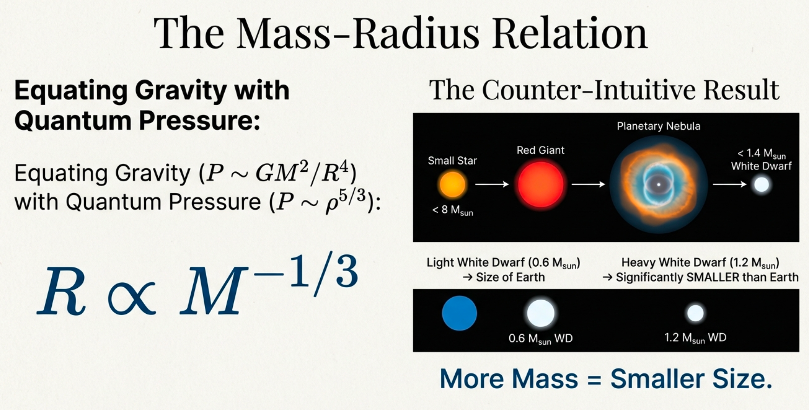
• Preview why white dwarfs get smaller when they gain mass (HW derivation)

No calculus. No memorizing formulas. Just dimensional logic.

4–5 min. Build anticipation. These are genuinely surprising results—especially the white dwarf one. Students should feel “I want to know how to do that.”

Vocabulary (define when needed later, not here):

• Event horizon = boundary beyond which nothing can escape; in GR language, no signals reach infinity.
• White dwarf = stellar remnant supported by electron degeneracy pressure.

About That “Math Person” Thing

You might be thinking: “I’m not a math person.”

Here’s the truth:

• Your brain physically changes when you learn hard things
• The discomfort you feel? That’s neurons forming new connections
• “Math person” is learned, not born—and it can be unlearned

This isn’t talent. It’s a skill you’re about to learn.

5–6 min. Keep brief but sincere. Reference “Why ASTR 201 is Different” if students have read it. The research is real (Moser et al., Woollett & Maguire).

The Challenge: Points of Light

Stars appear as mere points. Is that faint red glow a tiny nearby dwarf or a massive distant supergiant?

We can’t visit them. We can’t weigh them directly.

So how do we know anything about them?

We need a toolkit that extracts physics from limited data.

7–8 min. Quick transition. The hook already established the problem — now pivot to the solution.

Today’s Toolkit

Four methods that turn “points of light” into physics:

1. Dimensional Analysis — Is this equation even possible?
2. The Ratio Method — How does this compare to something known?
3. Unit Conversions — What’s the numeric value in useful units?
4. Order-of-Magnitude — Does this answer make sense?

These aren’t math drills—they’re inference tools.

Frame as empowerment. “You’re about to get superpowers.”

Why we’re doing this

Math as a telescope 🔭

Astronomy is the art of inferring physical reality from limited measurements.

Today’s superpower: units + dimensions catch mistakes before they become beliefs.

• We usually can’t touch the system — we observe light, motion, and time.
• We build simplified models that connect measurements to physics.
• We sanity-check (dimensions, units, scaling, limits) so we don’t compute nonsense confidently.

Emphasize: sanity-checking is not “extra,” it’s the job. Normalize struggle as part of modeling.

A quick disclaimer about “borrowed” equations

We will use a few equations before we derive them

Later this semester (and in your physics sequence) you’ll learn where they come from.

Rules for today

1. Treat them as reliable tools.
2. You do not need deep physical intuition yet.
3. You do need to know what each symbol means, and what the equation is claiming.

This slide prevents “but we haven’t learned this!” derailments and sets the epistemic norm: we can use trusted relations while building understanding over time.

How to read any equation (without panic)

The decoding ritual (we’ll use this all semester)

For any equation, ask:

1. What does it predict? (output)
2. What does it depend on? (inputs)
3. What happens if a variable increases? (direction + scaling)
4. What assumptions are hiding? (“only if…”)
5. Does it pass unit and limit checks?

Tell them: this is your “modeling checklist.” Repeat it often so it becomes automatic.

The four-tool workflow

Your survival kit 🧰

1. Dimensional analysis → “Could this formula possibly be right?”
2. Ratio method → “Compare without big-number pain.”
3. Unit conversion → “Translate SI ↔︎ CGS fluently.”
4. Order-of-magnitude → “Sanity-check reality.”

One sentence linking the tools: DA is structure, ratios cancel, unit conversion is language, OOM is plausibility.

Tool 1: Dimensional Analysis

The “smoke detector” for physics

Units vs. Dimensions

Credit: Course illustration (A. Rosen)

12–13 min. Key insight: units are human inventions, dimensions are physical reality.

The Fundamental Trio

Every physical quantity in this course is built from three ingredients:

Dimension	Symbol	Example (CGS)
Length	\([L]\)	cm
Mass	\([M]\)	g
Time	\([T]\)	s

Units are conventions (cm vs AU).

Dimensions are invariant physical DNA.

13–14 min. Emphasize: you can change units, but you can’t change what a quantity is. Press R twice to annotate Units then Dimensions.

Derived Quantities (CGS)

Quantity	Dimensions	CGS Unit
Velocity	\([LT^{-1}]\)	cm/s
Acceleration	\([LT^{-2}]\)	cm/s\(^2\)
Force	\([MLT^{-2}]\)	dyne (g cm/s\(^2\))
Energy	\([ML^2T^{-2}]\)	erg (g cm\(^2\)/s\(^2\))
Pressure	\([ML^{-1}T^{-2}]\)	dyne/cm\(^2\)

14–15 min. These are recipes. Energy = mass × length² / time².

Building Blocks

Credit: Course illustration (A. Rosen)

15–16 min. Visual equation builder. Note the sanity check box.

The Smoke Detector Test

If you calculate a star’s mass and your answer has dimensions of time…

The physics is wrong.

You don’t need a calculator to know something’s broken.

16–17 min. This catches errors before you waste time computing. The red highlight draws attention to the key insight.

Prediction: Dimensions of \(G\)

Newton’s law of gravity: \[F = \frac{GMm}{r^2}\]

What’s in this equation?

• \(F\): gravitational force between two masses
• \(G\): gravitational constant (how strong is gravity?)
• \(M\): mass of the central object (e.g., star)
• \(m\): mass of the orbiting object (e.g., planet with \(m \ll M\))
• \(r\): distance between the two masses

Before I show you: What dimensions must \(G\) have?

A. \([MLT^{-2}]\)   B. \([M^{-1}L^3T^{-2}]\)   C. \([L^3T^{-2}]\)   D. \([MT^{-2}]\)

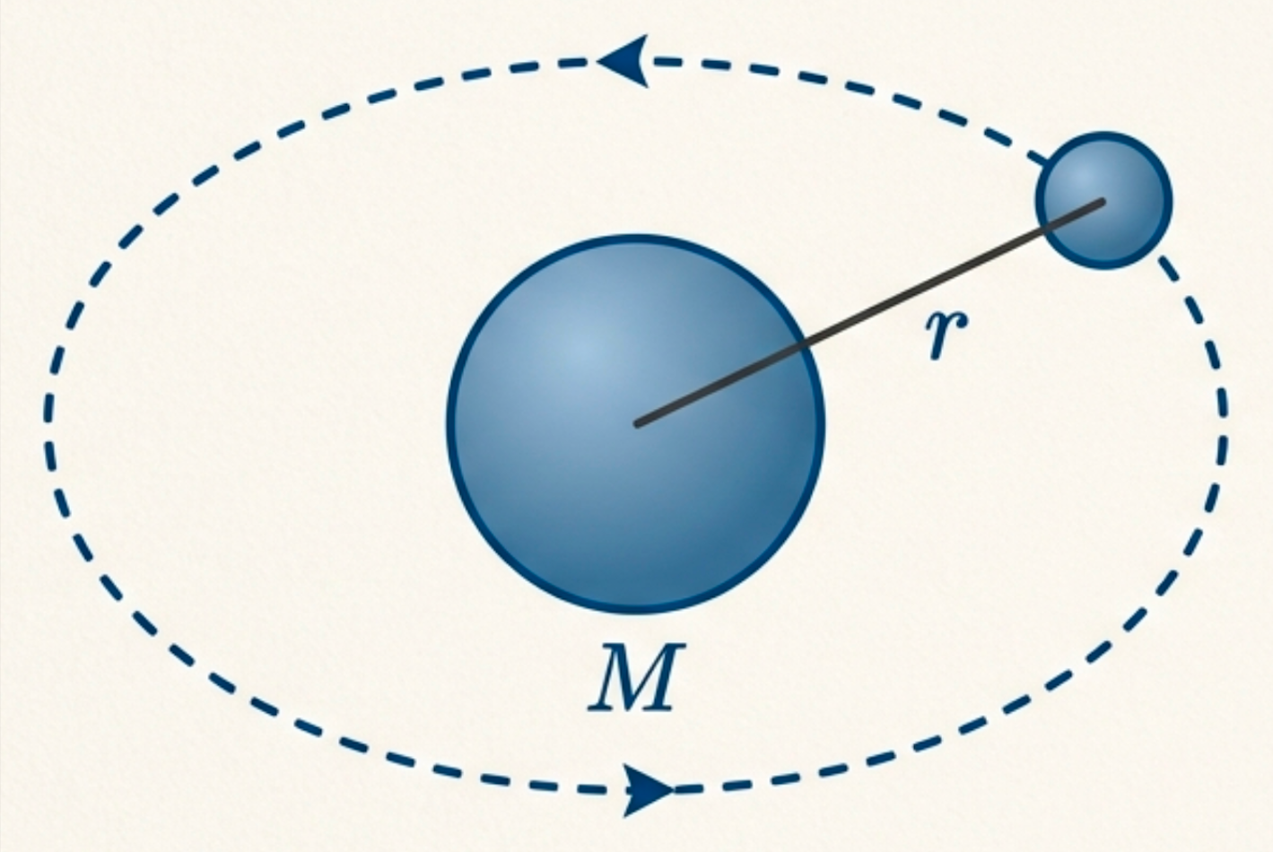
Give students 30 seconds. Cold-call or use iClicker. Common error: forgetting the inverse mass. Answer is B. Point to the figure: “This shows an orbit — \(M\) is the star, \(m\) is the planet, \(r\) is how far apart they are.”

Worked Example: What are the dimensions of \(G\)?

Newton’s law of gravity: \[F = \frac{GMm}{r^2}\]

Known dimensions:

• \([F] = MLT^{-2}\)
• \([M], [m] = M\)
• \([r] = L\)

Rearrange: \(G = \dfrac{F r^2}{M m}\)

\[ \begin{aligned} [G] &= \frac{[F][r]^2}{[M][m]} = \frac{(MLT^{-2})(L^2)}{M \cdot M} \\[0.5em] &= \frac{ML^3T^{-2}}{M^2} = M^{-1}L^3T^{-2} \\[0.5em] &\rightarrow \boxed{[G]= M^{-1}L^3T^{-2}} \end{aligned} \]

17–18 min. Walk through cancellation slowly. “G has composite units because it converts mass + distance into accelerations and timescales in Newton’s law.”

Constants Are Physical Quantities

Credit: Course illustration (A. Rosen)

18 min. Constants are not arbitrary numbers—they’re conversion factors built into the universe.

Check Yourself: Orbital Period

Kepler’s Third Law gives us: \[P \propto \sqrt{\frac{r^3}{GM}}\]

Question: Verify the dimensions work out to time \([T]\).

19 min. Give them 30 seconds to think.

Answer: \([r^3/GM] = [L^3]/[M^{-1}L^3T^{-2}][M] = [L^3]/[L^3T^{-2}] = [T^2]\)

Square root gives \([T]\). ✓

But Wait—How Did We Get That Formula?

We just verified Kepler’s Law.

But can we derive it from first principles?

Yes. Using only dimensional analysis.

The Protocol

19–20 min. This is the recipe. We’ll use it repeatedly.

Case A: Orbital period — setup

What can the orbital period depend on?

We want a formula for orbital period \(P\): “time for one orbit.”

Ingredients (allowed today):

• Orbit size \(r\) → \([L]\)
• Central mass \(M\) → \([M]\)
• Gravity constant \(G\) → \([M^{-1}L^{3}T^{-2}]\)

Goal: \[[P] = [T]\]

Equation meaning (gloss)

• \(P\): how long the orbit takes
• \(r\): how big the orbit is
• \(M\): how much mass is pulling
• \(G\): how strongly mass gravitates

20 min. Remind: we are NOT solving the orbit. We’re deducing how P scales with r and M.

Case A: Orbital period — solve (slow)

Assume: \(P \propto r^{a}M^{b}G^{c}\)

Convert to dimensions: \[[T] = [L]^a[M]^b[M^{-1}L^3T^{-2}]^c\] \[= [L]^{a+3c}[M]^{b-c}[T]^{-2c}\]

Match exponents:

• \(T:\; 1=-2c \Rightarrow c=-\tfrac12\)
• \(M:\; 0=b-c \Rightarrow b=-\tfrac12\)
• \(L:\; 0=a+3c \Rightarrow a=\tfrac32\)

\[\boxed{P \propto \sqrt{\frac{r^{3}}{GM}}}\]

20–21 min. Point out the “matching exponents” move explicitly. Students confuse units with dimensions—restate: [L] is “length-ness,” not meters specifically.

Case A: Orbital period — interpretation

\[P \propto \sqrt{\frac{r^{3}}{GM}}\]

• \(r \uparrow\) makes \(P\) grow fast: \(P \propto r^{3/2}\)
• \(M \uparrow\) makes \(P\) shrink: stronger gravity → faster orbit
• Unit check intuition: bigger distance → longer time ✅

What it predicts

Given \(r\), \(M\), \(G\), it predicts \(P\).

What it’s saying

“Farther orbits take much longer. More mass makes orbits faster.”

Optional “later this semester” add-on: \[P = 2\pi\sqrt{\frac{r^{3}}{GM}} \quad \text{(exact for circular orbits)}\]

21–22 min. Mention hidden assumptions: roughly circular orbit, central mass dominates, Newtonian gravity.

Stop & Solve 2: Ratio Method — Mars’ Year

Goal

Use ratios to avoid big-number arithmetic.

For planets orbiting the Sun, Kepler scaling gives: \[\left(\frac{P}{1\,\text{yr}}\right)^2=\left(\frac{a}{1\,\text{AU}}\right)^3\]

Mars has \(a = 1.52\,\text{AU}\).

1. Estimate \(P_{\text{Mars}}\) in years (1 significant figure is fine).
2. Write one sentence explaining why \(P\) grows faster than linearly with distance.

Hint: \(1.5^3 \approx 3.4\). Then take a square root.

→ Quick solution | → Detailed step-by-step

19–22 min (7–9 minutes total). - 2 min silent: compute rough \(1.52^3\) and sqrt. - 3 min pair: agree on estimate + interpretation sentence. - 2–3 min share: solicit 2 interpretations; correct gently. Emphasize: constants cancel; you’re using the solar system as a “calibration.” Navigation: Press G then type slide number to jump to solutions.

Stop & Solve 2 — Solution

\[\left(\frac{P}{1\,\text{yr}}\right)^2=\left(1.52\right)^3 \approx 3.5 \Rightarrow \frac{P}{1\,\text{yr}} \approx \sqrt{3.5}\approx 1.9\]

\[P_{\text{Mars}} \approx 1.9\,\text{yr}\]

Interpretation (sample): Farther orbits feel weaker gravity and have more distance to travel; the combination produces \(P \propto a^{3/2}\), so period grows quickly with distance.

← Back to problem | → Detailed solution

If students get ~2 years, celebrate. If they get ~3 years, it’s usually a squaring mistake; if they get ~1.2 years, they likely forgot the square root. Tie back to “scaling tells the story.”

Case B: Black hole horizon — setup

What sets the “point of no return”?

We want a characteristic radius \(R\) for a black hole (a length scale).

Ingredients:

• Mass \(M\) → \([M]\)
• Gravity \(G\) → \([M^{-1}L^3T^{-2}]\)
• Speed of light \(c\) → \([LT^{-1}]\)

Goal: \[[R]=[L]\]

Equation meaning (gloss)

• \(c\): speed limit of the universe
• if escape speed reaches \(c\), light can’t escape
• \(R\): the radius where that happens

28–29 min. Frame as “scale-setting”: we’re not doing GR, we’re figuring out how the size must scale with mass.

Case B: Black hole horizon — solve (slow)

Assume: \(R \propto G^{a}M^{b}c^{d}\)

(\(c = 3 \times 10^{8}\,\text{m/s}\), speed of light)

Dimensions: \[[L] = [M^{-1}L^3T^{-2}]^a[M]^b[LT^{-1}]^d\] \[= [L]^{3a+d}[M]^{-a+b}[T]^{-2a-d}\]

Match exponents:

• \(T:\;0=-2a-d \Rightarrow d=-2a\)
• \(M:\;0=-a+b \Rightarrow b=a\)
• \(L:\;1=3a+d \Rightarrow a=1\)

\[\boxed{R \propto \frac{GM}{c^2}}\]

Later-semester “exact” result (Schwarzschild): \(R_s=\frac{2GM}{c^2}\)

29–30 min. Reinforce: DA gives scaling, not factors of 2. Name “Schwarzschild radius” once (no deep dive).

Case B: Black hole horizon — interpretation

\[R_s=\frac{2GM}{c^2}\]

• \(M \uparrow\) → \(R_s \uparrow\) linearly
• bigger \(c\) would shrink horizons (faster universe makes trapping harder)
• this sets a length scale where escape becomes impossible

What it predicts

Given \(M\), it predicts the black hole’s horizon size.

What it’s saying

“More mass → bigger region where gravity wins against light.”

30 min. Call out assumptions gently: non-spinning/uncharged. Students love knowing there’s more complexity later.

Checkpoint 1 (retrieval)

1. If \(F \propto \dfrac{GMm}{r^2}\), what are the dimensions of \(F\)?
2. If the mass \(M\) doubles, how does \(R_s\) change?

Give 60–90 seconds silent think time. Then pair-share. Collect answers with a quick show-of-hands.

Checkpoint 1 — solutions

1. \([F] = [MLT^{-2}]\)
2. \(R_s \propto M\), so if \(M\) doubles, \(R_s\) doubles.

Make a point: “We did this without knowing any deep force law derivation—just dimensional consistency.”

White Dwarf Degeneracy Pressure (Teaser)

Credit: Course illustration (A. Rosen)

Homework teaser

You’ll get to try this derivation yourself on the homework: using dimensional + scaling logic to uncover why white dwarfs behave weirdly.

23–24 min. Optional in lecture (30–60 seconds): - Tease: quantum mechanics introduces \(\hbar\) → new “ingredient” sets pressure scale. - Do not derive live here; just frame it as “same toolkit, new physics ingredient.” Then move on to Tool 2.

The Counter-Intuitive Result (Teaser)

Credit: Course illustration (A. Rosen)

This is the punchline you’ll earn on HW

More mass → smaller white dwarf (until the Chandrasekhar limit). You’ll use the toolkit to see why that scaling emerges.

Keep it fast: promise payoff, don’t open the quantum rabbit hole. This makes the homework feel like a “mystery reveal,” not extra labor.

Tool 2: The Ratio Method

Escaping the “big number” trap

The Problem with Big Numbers

Mass of the Sun: \(M_\odot = 2 \times 10^{33}\) g Mass of the Earth: \(M_\oplus = 6 \times 10^{27}\) g

Subtraction fails

\[M_\odot - M_\oplus = 1.999... \times 10^{33} \text{ g}\]

Useless. Still a giant, meaningless number.

Division works

\[\frac{M_\odot}{M_\oplus} \approx 333{,}000\]

The Sun is 333,000× more massive than Earth.

Ratios give relative scale. Absolute numbers often don’t.

33–34 min. Key insight: ratios reveal physical relationships that raw numbers hide.

The Cancellation Trick

Most physical laws are proportionality relationships: \[A = kB^n\]

When comparing two systems: \[\frac{A_2}{A_1} = \frac{kB_2^n}{kB_1^n} = \left(\frac{B_2}{B_1}\right)^n\]

The constant \(k\) cancels!

We don’t need to know \(G\), \(\pi\), or \(\sigma\) numerically.

34–35 min. This is the key insight. Constants are “nuisances” that vanish in ratios.

Worked Example: Solar Volume

The Sun’s radius is 109 times Earth’s radius: \[\frac{R_\odot}{R_\oplus} = 109\]

Volume of a sphere: \(V = \frac{4}{3}\pi R^3\)

How many Earths fit inside the Sun?

\[\frac{V_\odot}{V_\oplus} = \left(\frac{R_\odot}{R_\oplus}\right)^3 = 109^3 \approx 1.3 \times 10^6\]

Over 1 million Earths!

35–36 min. Notice: we never calculated actual volumes in cm³. Ratios are enough.

Scaling Intuition

Scaling	Physical Meaning	Example
\(A \propto B^2\)	Area	Surface area, intensity
\(A \propto B^3\)	Volume	Mass (if density constant)
\(A \propto B^{-2}\)	Inverse-square	Gravity, light intensity

Small changes in input → big changes in output when \(n > 1\)

36–37 min. The power tells the physical story.

Concept Check: Surface Area Scaling

If you double a nebula’s radius, by what factor does its surface area increase?

• 2× (the radius doubled)
• 4× (surface area scales as R²)
• 8× (volume scaling)
• 16× (that would be R⁴)

Give students 30 seconds. Press C to reveal answer. Common error: choosing A (forgetting the square). Answer is B.

Solution: Surface Area

\[SA \propto R^2\] \[\frac{SA_2}{SA_1} = \left(\frac{2R}{R}\right)^2 = 4\]

Factor of 4. (The \(4\pi\) cancels.)

Tool 3: Unit Conversions

Why astronomers use CGS

First: Scientific Notation Crash Course

Numbers in astronomy get… absurd.

Mass of the Sun: \[1{,}989{,}000{,}000{,}000{,}000{,}000{,}000{,}000{,}000{,}000{,}000 \text{ g}\]

Nobody writes that. Instead:

\[M_\odot = 2 \times 10^{33} \text{ g}\]

38–39 min. This is the language of big (and small) numbers. Essential skill.

Reading Scientific Notation

\[a \times 10^n\]

Part	What it means
\(a\)	Coefficient (1–10)
\(10^n\)	“Move decimal \(n\) places”
\(n > 0\)	Big number (move right)
\(n < 0\)	Small number (move left)

Example: \(3.0 \times 10^{10}\) = 30,000,000,000 = 30 billion

39 min. The exponent tells you the magnitude. The coefficient is refinement.

Rules of the Game

Multiplication: Add exponents \[10^3 \times 10^5 = 10^{3+5} = 10^8\]

Division: Subtract exponents \[\frac{10^{33}}{10^{27}} = 10^{33-27} = 10^6\]

Powers: Multiply exponents \[(10^3)^2 = 10^{3 \times 2} = 10^6\]

39–40 min. These rules make astrophysical math manageable.

SI Prefixes: The Language of Scale

Prefix	Symbol	Power	Example
tera	T	\(10^{12}\)	THz (infrared)
giga	G	\(10^{9}\)	GHz (radio)
mega	M	\(10^{6}\)	Mpc (galaxy distances)
kilo	k	\(10^{3}\)	km (everyday)
centi	c	\(10^{-2}\)	cm (CGS!)
milli	m	\(10^{-3}\)	mm (wavelengths)
micro	μ	\(10^{-6}\)	μm (infrared)
nano	n	\(10^{-9}\)	nm (visible light)

40 min. You already know most of these! Astronomy just uses bigger/smaller ones.

Astronomy Lives at the Extremes

Scale	Value	Context
\(10^{-13}\) cm	Atomic nucleus	Where fusion happens
\(10^{-5}\) cm	Wavelength of light	What we detect
\(10^{10}\) cm	Solar radius	A typical star
\(10^{18}\) cm	1 parsec	Distance scale
\(10^{28}\) cm	Observable universe	Cosmic horizon

That’s 41 orders of magnitude. Scientific notation isn’t optional—it’s survival.

The CGS System

Astronomy uses CGS (centimeter-gram-second), not SI.

Base	CGS	SI
Length	cm	m
Mass	g	kg
Time	s	s

Derived units:

• Energy: erg (not Joule)
• Force: dyne (not Newton)
• Luminosity: erg/s (not Watt)

40–41 min. Historical convention that stuck. Numbers stay more manageable.

Why CGS?

SI (Physics textbooks)

\[L_\odot = 3.8 \times 10^{26} \text{ W}\]

CGS (Astrophysics)

\[L_\odot = 3.8 \times 10^{33} \text{ erg/s}\]

Both are correct. CGS is the community standard for astrophysics.

The Fractional Identity

The key insight: \(1 \text{ m} = 100 \text{ cm}\) means:

\[\frac{100 \text{ cm}}{1 \text{ m}} = 1\]

Multiplying by 1 doesn’t change the physics.

It only changes how we write the number.

34–35 min. Treat units like algebraic variables. They cancel.

Stop & Solve 3: Unit Conversions = Algebra

Goal

Convert units by multiplying by 1 (factor-label method).

3A. Speed (SI → CGS)

Convert \(30\,\mathrm{km/s}\) to \(\mathrm{cm/s}\). Show the chain: \[30\,\frac{\mathrm{km}}{\mathrm{s}} \times\frac{10^3\,\mathrm{m}}{1\,\mathrm{km}} \times\frac{10^2\,\mathrm{cm}}{1\,\mathrm{m}}\]

3B. Power / Luminosity units

Convert \(3.8\times 10^{26}\,\mathrm{W}\) to \(\mathrm{erg/s}\).

Given: \(1\,\mathrm{W}=1\,\mathrm{J/s}\), and \(1\,\mathrm{J}=10^7\,\mathrm{erg}\)

→ Quick solution | → Detailed 3A | → Detailed 3B

35–38 min (8–10 minutes total). - 3 min: do 3A individually (watch cancellation). - 3 min: do 3B in pairs. - 2–3 min: quick board solution; highlight “multiply by 1” mindset. Call out the classic trap: exponents apply to the conversion factor when units are squared/cubed. Navigation: Press G then type slide number to jump to solutions.

Stop & Solve 3 — Solution

3A

\[30\,\frac{\mathrm{km}}{\mathrm{s}} \times\frac{10^3\,\mathrm{m}}{1\,\mathrm{km}} \times\frac{10^2\,\mathrm{cm}}{1\,\mathrm{m}} =30\times 10^5\,\frac{\mathrm{cm}}{\mathrm{s}} =3\times 10^6\,\mathrm{cm/s}\]

3B

\[3.8\times 10^{26}\,\mathrm{W} =3.8\times 10^{26}\,\mathrm{J/s} =3.8\times 10^{26}\times 10^7\,\mathrm{erg/s} =3.8\times 10^{33}\,\mathrm{erg/s}\]

← Back to problem | → Detailed 3A | → Detailed 3B

Reinforce: the unit cancellation is the “proof.” Optional: ask them why CGS is convenient (community standard + fewer awkward prefixes in astro contexts).

Example 2: Energy (Exponents Matter!)

How many erg in 1 Joule?

\[1 \text{ J} = 1 \text{ kg} \cdot \text{m}^2 \cdot \text{s}^{-2}\]

\[= (10^3 \text{ g})(10^2 \text{ cm})^2 \text{ s}^{-2}\]

\[= 10^3 \times 10^4 \text{ g cm}^2 \text{ s}^{-2} = 10^7 \text{ erg}\]

48–49 min. Common mistake: forgetting to square the 100.

Example 3: The Stefan-Boltzmann Constant

SI: \(\sigma = 5.67 \times 10^{-8}\) W m\(^{-2}\) K\(^{-4}\)

Convert to CGS:

• W → erg/s: \(\times 10^7\)
• m\(^{-2}\) → cm\(^{-2}\): \(\times 10^{-4}\)

\[\sigma = 5.67 \times 10^{-8} \times 10^7 \times 10^{-4} = 5.67 \times 10^{-5} \text{ erg cm}^{-2} \text{ s}^{-1} \text{ K}^{-4}\]

Key Conversions to Memorize

Quantity	CGS Value
1 parsec	\(3.09 \times 10^{18}\) cm
1 AU	\(1.50 \times 10^{13}\) cm
Solar mass \(M_\odot\)	\(2.0 \times 10^{33}\) g
Solar radius \(R_\odot\)	\(7.0 \times 10^{10}\) cm
Solar luminosity \(L_\odot\)	\(3.8 \times 10^{33}\) erg/s

49–50 min. Pin these to your brain. You’ll use them constantly.

Tool 4: Order-of-Magnitude

The power of being “roughly right”

You Already Do This

“Can I drive there before dinner?”

You estimate:

• Distance: ~50 miles
• Speed: ~50 mph
• Time: ~1 hour

No calculator needed. Good enough.

51–52 min. Connect to everyday reasoning. This is natural.

Why It’s Essential in Astronomy

Numbers span 40+ orders of magnitude:

• Nucleus: \(10^{-13}\) cm
• Observable universe: \(10^{28}\) cm

Exact precision can hide the physics.

If you’re off by a factor of 2, that’s a triumph.

If you’re off by \(10^{10}\), something’s wrong.

The “Rule of 3”

When estimating:

• Coefficient \(< 3\) → round down to 1
• Coefficient \(> 3\) → round up to 10

Example:

• \(2 \times 10^{33}\) → \(10^{33}\)
• \(7 \times 10^{10}\) → \(10^{11}\)

52–53 min. The exponent tells the story. Coefficients are refinement.

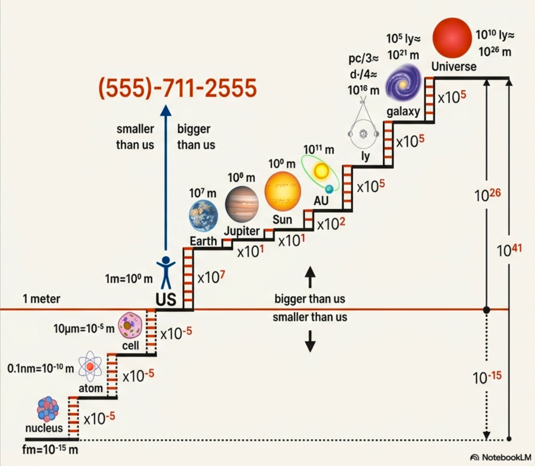
The Universe’s Phone Number

Credit: Fundamentals of Astrophysics (Owocki)

53–54 min. The staircase shows each multiplication factor. The phone number encodes the jumps between scales. Have students write this down—they’ll use it as a sanity check all semester.

Cosmic Scales: Powers of 10

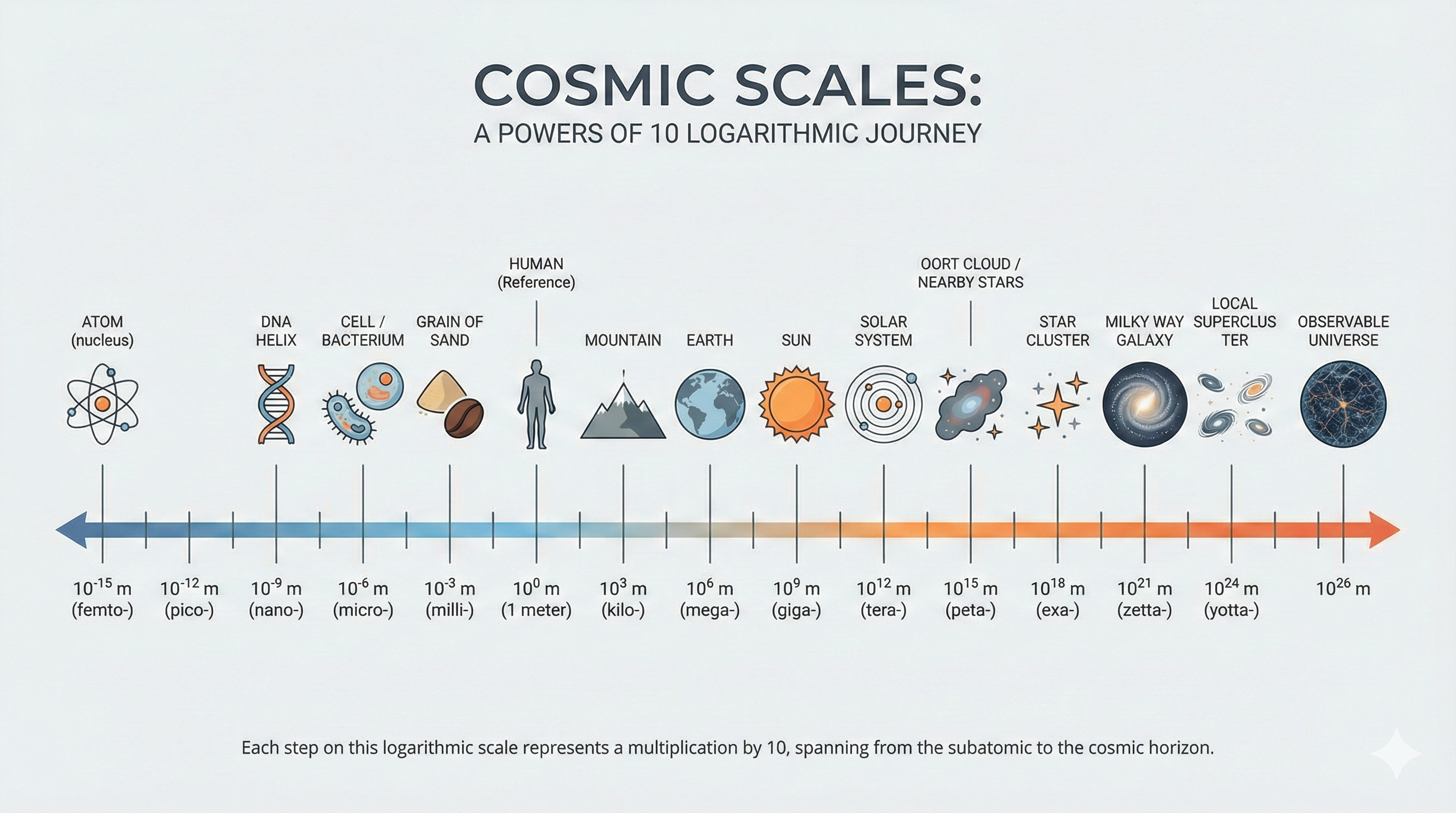
Credit: Gemini

54 min. Another visualization of the same idea. Each step is ×10. Human scale sits in the middle. Point out that we’re roughly halfway between nucleus and universe on a log scale.

Reading the Phone Number

Area Code (555): Three steps DOWN from human scale

• × \(10^{-5}\) : human → cells
• × \(10^{-5}\) : cells → atoms
• × \(10^{-5}\) : atoms → nucleus

Exchange (711): Solar system

• × \(10^{7}\) : human → Earth
• × \(10^{1}\) : Earth → Jupiter
• × \(10^{1}\) : Jupiter → Sun

Reading the Phone Number (cont.)

Subscriber (2555): Cosmos

• × \(10^{2}\) : Sun → 1 AU (Earth–Sun distance)
• × \(10^{5}\) : 1 AU → nearest stars (~1 pc)
• × \(10^{5}\) : nearest stars → Milky Way
• × \(10^{5}\) : Milky Way → observable universe

If your calculation gives stellar distance = \(10^{11}\) cm…

That’s Sun-sized, not star-distance. Red flag!

Everyday Example: Piano Tuners in Chicago

How many piano tuners work in Chicago?

• Population: ~3 million → \(10^6\)
• Pianos per household: ~1/20 → \(10^{-1}\)
• Tunings per piano per year: ~1
• Tunings per tuner per year: ~500 → \(10^3\)

\[\frac{10^6 \times 10^{-1} \times 1}{10^3} = 10^2 \approx 100\text{–}300 \text{ tuners}\]

54–55 min. Classic Fermi problem. We got ballpark without exact data.

Stop & Solve 4: OOM + Scaling — Black Hole Sizes

Goal

Use a known anchor + scaling to stay in the right powers-of-ten “zip code.”

Assume:

• A 1 \(M_\odot\) black hole has \(R_s \approx 3\,\mathrm{km}\).
• \(R_s\) scales linearly with mass: \(R_s \propto M\).

1. Estimate \(R_s\) for a 10 \(M_\odot\) black hole.
2. Estimate \(R_s\) for a 4 million \(M_\odot\) black hole (Sgr A* scale).
3. Convert #2 to scientific notation (km), then decide: closer to
   • Earth size (\(\sim 10^4\) km),
   • Sun size (\(\sim 10^6\) km),
   • or AU size (\(\sim 10^8\) km)?

→ Quick solution | → Detailed step-by-step

44–47 min (8–10 minutes total). - 2 min silent: #1 and #2. - 2–3 min pair: #3 classification argument. - 3–4 min share: get multiple answers; focus on order-of-magnitude reasoning. Key message: you can get powerful insight from one anchor value + proportionality. Navigation: Press G then type slide number to jump to solutions.

Stop & Solve 4 — Solution

Since \(R_s \propto M\):

1. 10 \(M_\odot\): \[R_s \approx 3\,\mathrm{km}\times 10 \approx 30\,\mathrm{km}\]

2. \(4\times 10^6\,M_\odot\): \[R_s \approx 3\,\mathrm{km}\times 4\times 10^6 \approx 1.2\times 10^7\,\mathrm{km}\]

3. Comparison: \[1.2\times 10^7\,\mathrm{km}\] is bigger than Sun-scale (\(\sim 10^6\) km) and smaller than AU-scale (\(\sim 10^8\) km) — closer to AU than to the Sun, but still within an order of magnitude of “solar system” scales.

← Back to problem | → Detailed solution

This is a great moment to remind them: black holes are compact per unit mass, but supermassive ones are still physically enormous in km. If students got ~\(10^7\) km, celebrate! That’s Sgr A* — about \(0.08\) AU, well inside Mercury’s orbit.

Bonus: Verify the Anchor Value

Where did \(R_s \approx 3\) km come from? Use \(R_s \approx \frac{GM}{c^2}\)

CGS values:

• \(G \approx 10^{-7}\,\frac{\text{cm}^3}{\text{g}\cdot\text{s}^{2}}\)
• \(M_\odot \approx 10^{33}\,\text{g}\)
• \(c \approx 10^{10}\,\frac{\text{cm}}{\text{s}}\)

Substitute: \[R_s \approx \frac{10^{-7} \cdot 10^{33}}{(10^{10})^2}\,\frac{\text{cm}^3 \cdot \cancel{\text{g}} \cdot \cancel{\text{s}^{2}}}{\cancel{\text{g}} \cdot \cancel{\text{s}^{2}} \cdot \text{cm}^2}\]

\[= \frac{10^{26}}{10^{20}}\,\text{cm} = 10^{6}\,\text{cm} = 10\,\text{km}\]

Exact: 3 km. Factor of 3 off — OOM success!

Connecting the Toolkit

The Problem-Solving Flow

flowchart LR
    A[Question] --> B[Dimensional Analysis]
    B -->|Valid?| C[Ratio Method]
    C -->|Compare| D[Unit Conversion]
    D -->|Calculate| E[OOM Check]
    E -->|Sensible?| F[Answer]

Use all four tools together for robust reasoning.

Your New Superpowers

Tool	Question It Answers
Dimensional Analysis	Is this equation physically valid?
Ratio Method	How does this compare to something known?
Unit Conversions	What’s the numeric value in CGS?
OOM Estimation	Does this answer make sense?

The Toolbox

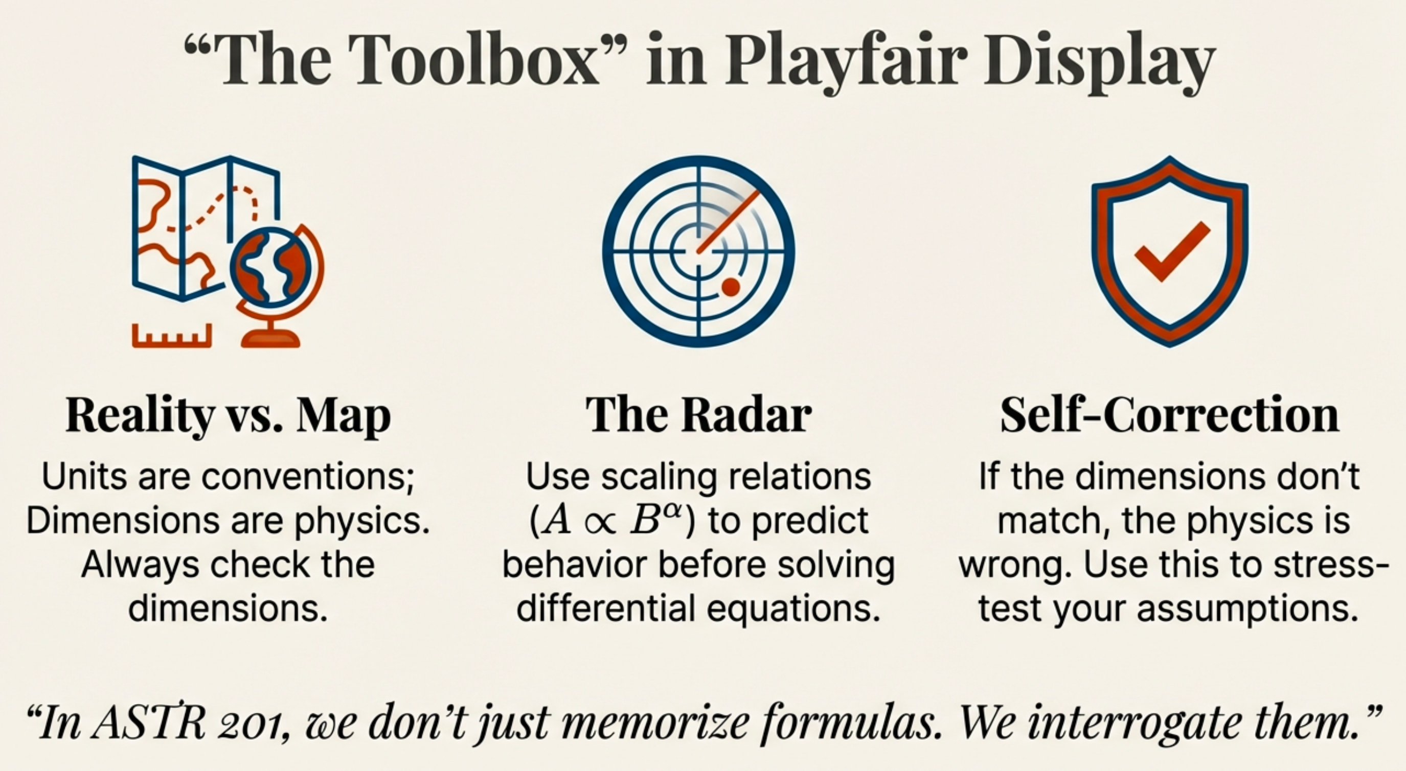
Credit: Course illustration (A. Rosen)

Key message: We don’t just memorize formulas. We interrogate them.

Preview: Where You’ll Use These

• Module 2: Stellar distances → ratios everywhere
• Module 3: Stellar structure → dimensional scaling
• Module 4: Cosmology → OOM across the universe

These tools are your scientific radar for the rest of the course.

One Thing to Remember

The Takeaway

If you forget everything else from today, remember this:

Dimensions are your smoke detector.

Before trusting any equation, check that both sides have the same dimensions.

If they don’t match, the physics is guaranteed to be wrong.

63–64 min. This is the core message. Emphasize: dimensional analysis catches errors before they cost you time and points. The fade-up animation and fit-text make this memorable.

Questions?

Common questions at this point:

• “What counts as showing work on homework?”
• “How strict are you about units?”
• “Do we need to memorize the phone number?”

64–65 min. Address these directly. Work = show dimensional analysis. Units = CGS always. Phone number = useful mnemonic, not required.

Solutions Reference

Detailed step-by-step solutions for self-study

These slides are for students to review after class, or for you to jump to if you want to show complete worked solutions. Press G then type slide number to jump quickly.

Solution 1: Dimensional Detective — Full Work

Setup

Given: Four candidate formulas for orbital period \(P\)

Find: Which have dimensions of time \([T]\)

Key fact: \([G] = [M^{-1}L^3T^{-2}]\), so \([GM] = [L^3T^{-2}]\)

Option 1: \(P \propto \dfrac{r^2}{GM}\)

\[\left[\frac{r^2}{GM}\right] = \frac{[L]^2}{[L^3T^{-2}]} = \frac{[L^2]}{[L^3][T^{-2}]} = [L^{2-3}][T^{+2}] = [L^{-1}T^2]\]

\[\boxed{\text{Not } [T] \text{ — WRONG}}\]

→ Back to problem

Solution 1 (cont.) — Options 2–4

Option 2: \(P \propto \sqrt{\dfrac{r^3}{GM}}\)

\[\left[\sqrt{\frac{r^3}{GM}}\right] = \sqrt{\frac{[L^3]}{[L^3T^{-2}]}} = \sqrt{\frac{[L^3]}{[L^3]}\cdot[T^2]} = \sqrt{[T^2]} = [T] \quad \boxed{\checkmark \text{ CORRECT}}\]

Option 3: \(P \propto \dfrac{r}{\sqrt{GM}}\)

\[\left[\frac{r}{\sqrt{GM}}\right] = \frac{[L]}{\sqrt{[L^3T^{-2}]}} = \frac{[L]}{[L^{3/2}T^{-1}]} = [L^{1-3/2}][T^1] = [L^{-1/2}T] \quad \boxed{\text{WRONG}}\]

Option 4: \(P \propto \sqrt{\dfrac{GM}{r^3}}\)

\[\left[\sqrt{\frac{GM}{r^3}}\right] = \sqrt{\frac{[L^3T^{-2}]}{[L^3]}} = \sqrt{[T^{-2}]} = [T^{-1}] \quad \boxed{\text{WRONG (frequency, not period)}}\]

Solution 2: Mars Year — Full Work

Setup

Given: Mars orbital distance \(a = 1.52\) AU Find: Mars orbital period \(P\) in years Formula: \(\left(\dfrac{P}{1\,\text{yr}}\right)^2 = \left(\dfrac{a}{1\,\text{AU}}\right)^3\) (Kepler’s Third Law)

Step 1: Substitute known value \[\left(\frac{P}{1\,\text{yr}}\right)^2 = (1.52)^3\]

Step 2: Evaluate the cube (show your work!) \[1.52^3 = 1.52 \times 1.52 \times 1.52 = 2.31 \times 1.52 \approx 3.51\]

Step 3: Take square root of both sides \[\frac{P}{1\,\text{yr}} = \sqrt{3.51} \approx 1.87\]

Step 4: Solve for \(P\) \[\boxed{P_{\text{Mars}} \approx 1.9 \text{ years}}\]

Actual value: 1.88 years — excellent agreement!

→ Back to problem

Solution 2 (cont.) — Why \(P \propto a^{3/2}\)?

Physical interpretation:

A planet farther from the Sun experiences two effects:

1. Longer path: Circumference \(\propto a\), so more distance to travel
2. Weaker gravity: Force \(\propto 1/a^2\), so slower orbital speed

Combined effect: \(P \propto a^{3/2}\) — period grows faster than linearly with distance.

Sanity check

• Earth at 1 AU: \(P = 1\) yr ✓
• Mars at 1.52 AU: \(P \approx 1.9\) yr ✓ (farther → longer)
• Jupiter at 5.2 AU: \(P = 5.2^{1.5} \approx 12\) yr ✓

Solution 3A: Speed Conversion — Full Work

Setup

Given: Earth’s orbital speed = \(30\) km/s Find: Speed in cm/s (CGS) Method: Multiply by conversion factors = 1

Step 1: Write conversion factors \[1\,\text{km} = 10^3\,\text{m} \quad \Rightarrow \quad \frac{10^3\,\text{m}}{1\,\text{km}} = 1\] \[1\,\text{m} = 10^2\,\text{cm} \quad \Rightarrow \quad \frac{10^2\,\text{cm}}{1\,\text{m}} = 1\]

Step 2: Chain the conversions (watch units cancel!) \[30\,\frac{\cancel{\text{km}}}{\text{s}} \times \frac{10^3\,\cancel{\text{m}}}{1\,\cancel{\text{km}}} \times \frac{10^2\,\text{cm}}{1\,\cancel{\text{m}}} = 30 \times 10^3 \times 10^2 \,\frac{\text{cm}}{\text{s}}\]

Step 3: Combine powers of 10 \[= 30 \times 10^{3+2}\,\text{cm/s} = 30 \times 10^5\,\text{cm/s} = \boxed{3 \times 10^6\,\text{cm/s}}\]

→ Back to problem

Solution 3B: Luminosity Conversion — Full Work

Setup

Given: \(L_\odot = 3.8 \times 10^{26}\) W (SI) Find: \(L_\odot\) in erg/s (CGS) Key conversion: \(1\,\text{W} = 1\,\text{J/s}\) and \(1\,\text{J} = 10^7\,\text{erg}\)

Step 1: Expand Watts to fundamental units \[3.8 \times 10^{26}\,\text{W} = 3.8 \times 10^{26}\,\frac{\text{J}}{\text{s}}\]

Step 2: Convert Joules to ergs \[= 3.8 \times 10^{26}\,\frac{\cancel{\text{J}}}{\text{s}} \times \frac{10^7\,\text{erg}}{1\,\cancel{\text{J}}}\]

Step 3: Combine powers of 10 \[= 3.8 \times 10^{26} \times 10^7\,\frac{\text{erg}}{\text{s}} = 3.8 \times 10^{26+7}\,\text{erg/s}\]

\[\boxed{L_\odot = 3.8 \times 10^{33}\,\text{erg/s}}\]

Common error: Forgetting that 1 J = \(10^7\) erg (not \(10^3\)!). Energy in CGS uses small units.

Solution 4: Black Hole Scaling — Full Work

Setup

Given: \(R_s(1\,M_\odot) \approx 3\) km (anchor value) Scaling law: \(R_s \propto M\) (linear) Find: \(R_s\) for 10 \(M_\odot\) and \(4 \times 10^6\,M_\odot\)

Part 1: Stellar-mass black hole (10 \(M_\odot\)) \[\frac{R_s(10\,M_\odot)}{R_s(1\,M_\odot)} = \frac{10\,M_\odot}{1\,M_\odot} = 10\]

\[R_s(10\,M_\odot) = 10 \times 3\,\text{km} = \boxed{30\,\text{km}}\]

Part 2: Supermassive black hole (\(4 \times 10^6\,M_\odot\), like Sgr A*) \[\frac{R_s(4\times10^6\,M_\odot)}{R_s(1\,M_\odot)} = \frac{4\times10^6\,M_\odot}{1\,M_\odot} = 4\times10^6\]

\[R_s = (4\times10^6) \times 3\,\text{km} = 12\times10^6\,\text{km} = \boxed{1.2\times10^7\,\text{km}}\]

→ Back to problem

Solution 4 (cont.) — Scale Comparison

Part 3: How big is \(1.2 \times 10^7\) km?

Object	Size
Earth radius	\(6.4 \times 10^3\) km
Sun radius	\(7 \times 10^5\) km
Sgr A* horizon	\(1.2 \times 10^7\) km
Mercury’s orbit	\(5.8 \times 10^7\) km
1 AU	\(1.5 \times 10^8\) km

\[\boxed{\text{Sgr A* is about 17× the Sun's radius, or } \sim 0.08 \text{ AU}}\]

Sanity check

• Bigger than Sun? ✓ (by factor ~17)
• Smaller than 1 AU? ✓ (by factor ~12)
• Sgr A’s horizon (~0.08 AU) fits well inside* Mercury’s orbit (~0.39 AU)

Problem-Solving Best Practices

The Template

Every solution should follow this structure:

1. Setup box: State what’s given and what you’re finding
2. Write the formula: Include units/dimensions
3. Substitute: Put numbers in, keep units attached
4. Cancel units: Cross out matching units explicitly
5. Compute: Show exponent arithmetic (\(10^a \times 10^b = 10^{a+b}\))
6. Box the answer: With units!
7. Sanity check: Does the answer make physical sense?

Common pitfalls

• Dropping units mid-calculation
• Forgetting to square/cube conversion factors
• Not checking if answer is in the right “ballpark”

Reference Tables

See the Lecture 2 Reference Handout for:

• CGS unit conversions
• Fundamental physical constants
• Solar units (\(M_\odot\), \(R_\odot\), \(L_\odot\))
• Key distance scales (AU, pc)
• Dimensional “recipes”

Direct students to the handout. They should keep it handy for homework.