Lecture 4 (Day 2):
Light as Information

Models • Spectral Fingerprints • Telescopes

Dr. Anna Rosen

February 5, 2026

Learning Objectives

By the end of today, you will be able to:

• Use limiting-case reasoning to interpret the shape of a blackbody spectrum (Rayleigh–Jeans vs Wien tail)
• Explain why atoms produce absorption and emission lines and identify the three spectrum types (Kirchhoff)

Learning Objectives (continued)

• Describe how a real stellar spectrum combines continuum + lines
• Apply the two key telescope scalings: collecting area \(\propto D^2\) and resolution \(\propto \lambda D^{-1}\)
• Apply the Doppler equation to connect line shifts to radial velocity

Day 2 cohesion: Day 1 gave us the foundation — light is waves + particles, and temperature sets color via Wien. Today we read that color (limiting cases make Planck tractable) AND add fine structure: spectral lines encode composition, Doppler encodes motion. This completes the “light as information” toolkit.

Today is “how we read spectra” + “why instruments matter”.

Same object.

Different wavelength.

Different story.

This is the motivation for “spectrum + instruments”.

Today’s Game Plan

We finish the “radiation foundation” in three moves:

1. Why the blackbody curve has simple limits (so we can use it)
2. How atoms add spectral lines (so we can infer composition)
3. How telescopes change what we can measure (photons + resolution)

Make this explicit: today is not “more facts” — it’s “how to read spectra like an astronomer”.

Quick Recall (Day 1)

Fill in the blanks:

• Waves: \(c = \lambda\nu\)
• Photons: \(E = hc\lambda^{-1}\)
• Thermal peak: \(\lambda_{\mathrm{peak}} \propto T^{-1}\)

Let students say them out loud. Remind: we are building an inference toolkit.

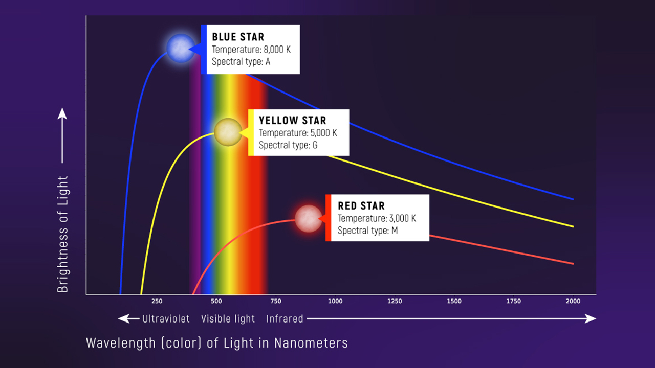
🧠 Quiz: Temperature from Color

A thermal spectrum peaks at a shorter wavelength. The object is…

• hotter
• cooler
• the same temperature
• necessarily younger

Answer: hotter. This is Wien’s law in action: \(\lambda_{\text{peak}} \propto T^{-1}\). Shorter peak wavelength means higher temperature. “Necessarily younger” is a distractor — age and temperature are not directly related (old stars can be hot, young stars can be cool depending on mass).

Planck + Wien (Thermal Equilibrium)

Thermal equilibrium means energy absorbed equals energy emitted, so the temperature is stable and the spectrum depends only on \(T\).

Planck function (blackbody spectrum)

What it predicts
Spectral radiance \(B_\lambda\) of a blackbody as a function of wavelength.

What it depends on
Wavelength \(\lambda\) and temperature \(T\), with constants \(h\), \(c\), and \(k_B\).

What it's saying
Two factors compete: the \(\lambda^{-5}\) term pushes short wavelengths up, while the exponential term suppresses them. Because \(h\nu\) and \(k_B T\) are both energies, the ratio \(h\nu/k_B T\) (or \(hc/\lambda k_B T\)) is dimensionless and sets the regime: \(h\nu \ll k_B T\) → Rayleigh–Jeans power law; \(h\nu \gg k_B T\) → Wien tail.

Assumptions

• Object radiates as an ideal blackbody in thermal equilibrium
• Spectrum expressed per unit wavelength interval

See: the equation

Wien’s law anchors the peak wavelength:

\[ \lambda_{\text{peak}} = b T^{-1} \tag{1}\]

Use this to name what “thermal equilibrium” buys us: a single-parameter spectrum.

Part 1: The Planck Curve Has “Handlebars”

Limiting cases make scary equations usable.

The Story Behind the Curve

Classically, you might expect short wavelengths to dominate because:

• shorter \(\lambda\) often means higher energy per photon
• power laws like \(\lambda^{-4}\) rise fast as \(\lambda\) shrinks

Set up the “failure mode” before naming it.

The Ultraviolet Catastrophe (What Went Wrong)

Classical physics predicts a spectrum that blows up at short wavelength.

That would mean infinite energy in the ultraviolet.

Reality: the spectrum peaks and then drops.

No numbers. Just the conceptual mismatch: classical → divergence; reality → peak + cutoff.

Planck’s Quantum Move

Energy is emitted/absorbed in chunks:

\[E = h\nu\]

• high frequency (short \(\lambda\)) photons cost more energy per photon
• at a given \(T\), very high-energy photons are rare

Tie to Day 1: this is why “very high-energy photons are expensive.”

The Planck Function (Recognize It)

You don’t memorize it — you recognize it and read its structure:

\[ B_\lambda(T)=\frac{2hc^2}{\lambda^5}\cdot\frac{1}{e^{hc/(\lambda k_B T)}-1} \tag{2}\]

• \(B_\lambda\): spectral radiance (brightness per wavelength interval)
• \(\lambda\): wavelength, \(T\): temperature
• Units: erg·s\(^{-1}\)·cm\(^{-2}\)·sr\(^{-1}\)·cm\(^{-1}\)

Credit: JWST/STScI

One sentence: this is the quantitative model behind the curves. Do not dwell on constants; we’re here for interpretation.

How to Read \(B_\lambda(T)\) (Study Version)

Read it like a sentence:

Planck function (blackbody spectrum)

What it predicts
Spectral radiance \(B_\lambda\) of a blackbody as a function of wavelength.

What it depends on
Wavelength \(\lambda\) and temperature \(T\), with constants \(h\), \(c\), and \(k_B\).

What it's saying
Two factors compete: the \(\lambda^{-5}\) term pushes short wavelengths up, while the exponential term suppresses them. Because \(h\nu\) and \(k_B T\) are both energies, the ratio \(h\nu/k_B T\) (or \(hc/\lambda k_B T\)) is dimensionless and sets the regime: \(h\nu \ll k_B T\) → Rayleigh–Jeans power law; \(h\nu \gg k_B T\) → Wien tail.

Assumptions

• Object radiates as an ideal blackbody in thermal equilibrium
• Spectrum expressed per unit wavelength interval

See: the equation

This is the “equation contract” slide without the full derivation.

How to Read the Curve (Where the Limits Live)

Use the curve as your map:

• Right side (long \(\lambda\)): \(h\nu \ll k_B T\) → Rayleigh–Jeans power law
• Left side (short \(\lambda\)): \(h\nu \gg k_B T\) → Wien exponential drop

Credit: JWST/STScI

Point to the curve: right side is the “low-energy photons” regime; left side is the “high-energy photons are rare” regime.

You Don’t Memorize Planck — You Read It

The blackbody curve has two key regimes:

• Long-wavelength tail (Rayleigh–Jeans)
• Short-wavelength tail (Wien)

Those regimes let you predict behavior without re-deriving the whole function.

Credit: JWST/STScI

What the Planck Function Does

Even without memorizing it, recognize the structure:

\[ B_\lambda(T)=\frac{2hc^2}{\lambda^5}\cdot\frac{1}{e^{hc/(\lambda k_B T)}-1} \tag{3}\]

• power‑law prefactor (\(2hc^2/\lambda^5\)) rises steeply toward short \(\lambda\)
• exponential term (\(e^{hc/\lambda k_B T}\)) suppresses short \(\lambda\)
• because \(h\nu\) and \(k_B T\) are both energies, \(h\nu/k_B T\) is the dimensionless “regime knob”

Credit: JWST/STScI

This mirrors the reading’s “structure” section: power-law vs exponential.

Long Wavelengths (Rayleigh–Jeans Limit)

At long wavelengths, the spectrum behaves like:

\[B_\lambda \propto T\lambda^{-4}\]

• at fixed \(\lambda\): hotter → brighter (linear in \(T\))
• at fixed \(T\): shorter \(\lambda\) → much brighter (\(\lambda^{-4}\) is steep)

Connect to Rayleigh scattering’s “steep power law” vibe — steep exponents matter.

Where Does Rayleigh–Jeans Apply?

Rayleigh–Jeans is a long-wavelength approximation.

• Condition: \(h\nu \ll k_B T\)
• On the curve, it’s the right side of the peak (long \(\lambda\)).

Credit: JWST/STScI

This prevents over-applying power laws where the exponential cutoff matters.

🧠 Predict (Rayleigh–Jeans)

Rayleigh–Jeans: \(B_\lambda \propto T\lambda^{-4}\) (long \(\lambda\), \(h\nu \ll k_B T\)).

At fixed temperature, if wavelength doubles, \(B_\lambda\) changes by…

• \(\times 2\)
• \(\times 4\)
• \(\times 8\)
• \(\div 16\)

Short Wavelengths (Wien Tail)

At short wavelengths, the spectrum drops off exponentially:

\[B_\lambda \approx \left(\text{power law}\right)\times e^{-hc/\lambda k_B T}\]

Interpretation: very high-energy photons are “expensive” thermally.

No derivation. Just the story: exponential suppression at short wavelength.

Where Does the Wien Tail Apply?

The Wien tail is the short-wavelength side of the curve.

• Condition: \(h\nu \gg k_B T\)
• On the curve, it’s the left side of the peak (short \(\lambda\)).

That’s why hot objects can emit UV, but not “infinite UV.”

Credit: JWST/STScI

What Limiting Cases Buy Us

Instead of memorizing a complicated formula, we can answer questions like:

• “Which side of the peak am I on?”
• “Does intensity fall as a power law or exponentially?”
• “What changes faster: with \(T\) or with \(\lambda\)?”

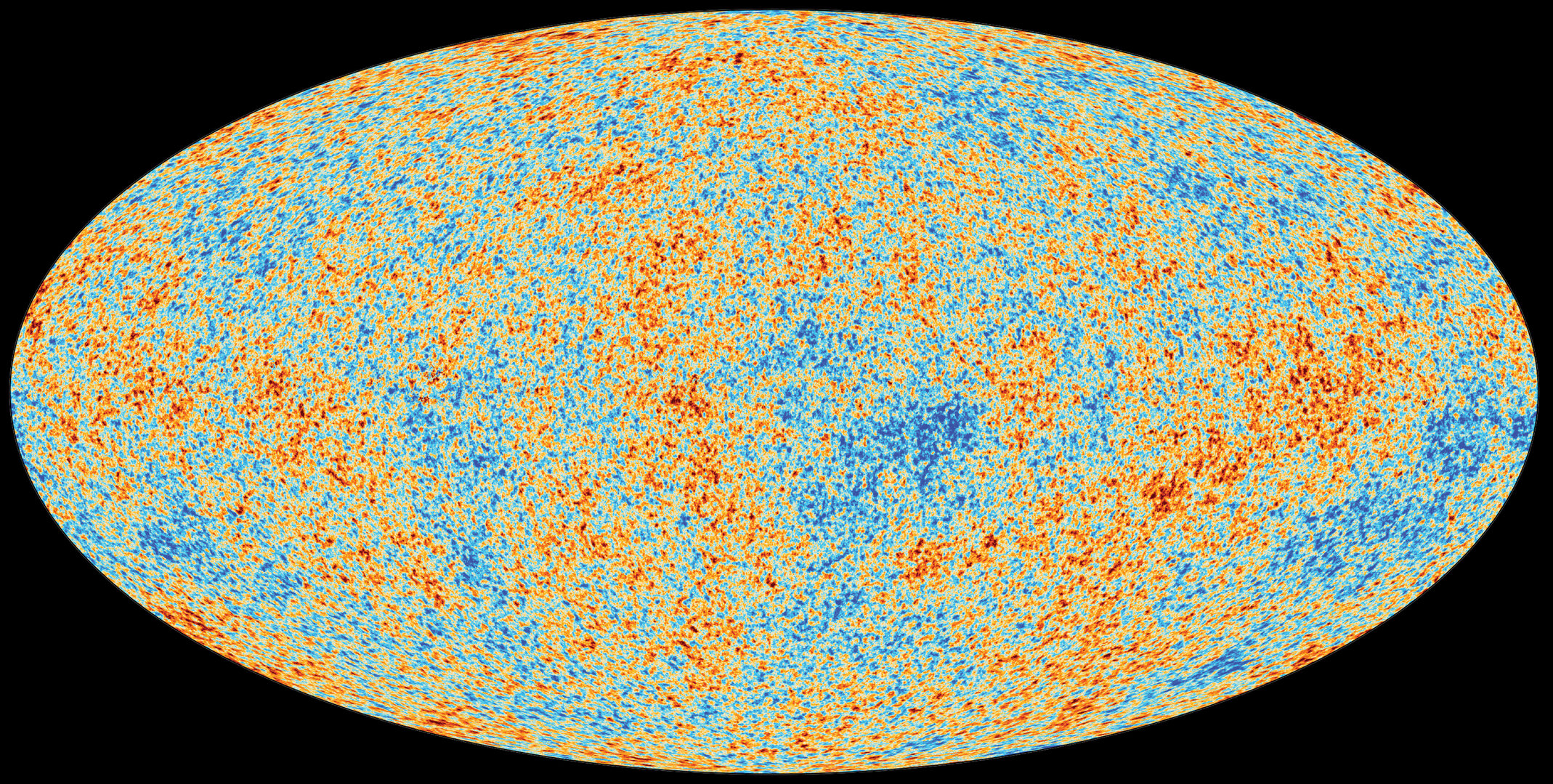
Example: The Cosmic Microwave Background

The CMB is an almost perfect blackbody:

• temperature \(\approx 2.725\ \mathrm{K}\)
• peak is in the microwave

It’s “thermal radiation from the early universe,” stretched and cooled by cosmic expansion.

A tiny part of old analog TV “snow” was this same microwave background — a faint hiss from the early universe.

Credit: ESA/Planck Collaboration

Do not go deep into cosmology here. Use it as: “blackbodies aren’t only stars.”

CMB: Quick Peak Estimate (Fast Math)

Using Wien’s law with \(T\approx 2.7\ \mathrm{K}\):

\[ \begin{aligned} \lambda_{\mathrm{peak}} &\approx \frac{0.29\ \text{cm}\cdot\text{K}}{2.7\ \text{K}} \\ &= \left(\frac{0.29}{2.7}\right)\ \text{cm} \\ &\approx 0.11\ \text{cm} \\ &= 1.1\ \text{mm} \end{aligned} \]

That’s about a millimeter → microwave.

A Subtle Plotting Warning (Optional)

The “peak wavelength” depends on whether you plot:

• \(B_\lambda\) (per wavelength interval), or
• \(B_\nu\) (per frequency interval)

Same physics; different axis choice can shift where the peak appears.

This matches the reading’s “Representation Warning.” Tell them: you’ll always specify which is being used.

Part 2: Spectral Lines = Atomic Fingerprints

Continuum tells temperature; lines tell composition.

Why Lines Exist (One Sentence)

Atoms have quantized energy levels — they absorb or emit photons with specific energies.

Name the misconception: “atoms can absorb any wavelength”. No: only what matches energy gaps.

The Bohr Model (A First Mental Picture)

Electrons live on “allowed steps” (energy levels).

• jump up → absorb a photon
• fall down → emit a photon

Goal: quantization as a model. Don’t pretend it’s the full modern picture; it’s the simplest useful scaffold.

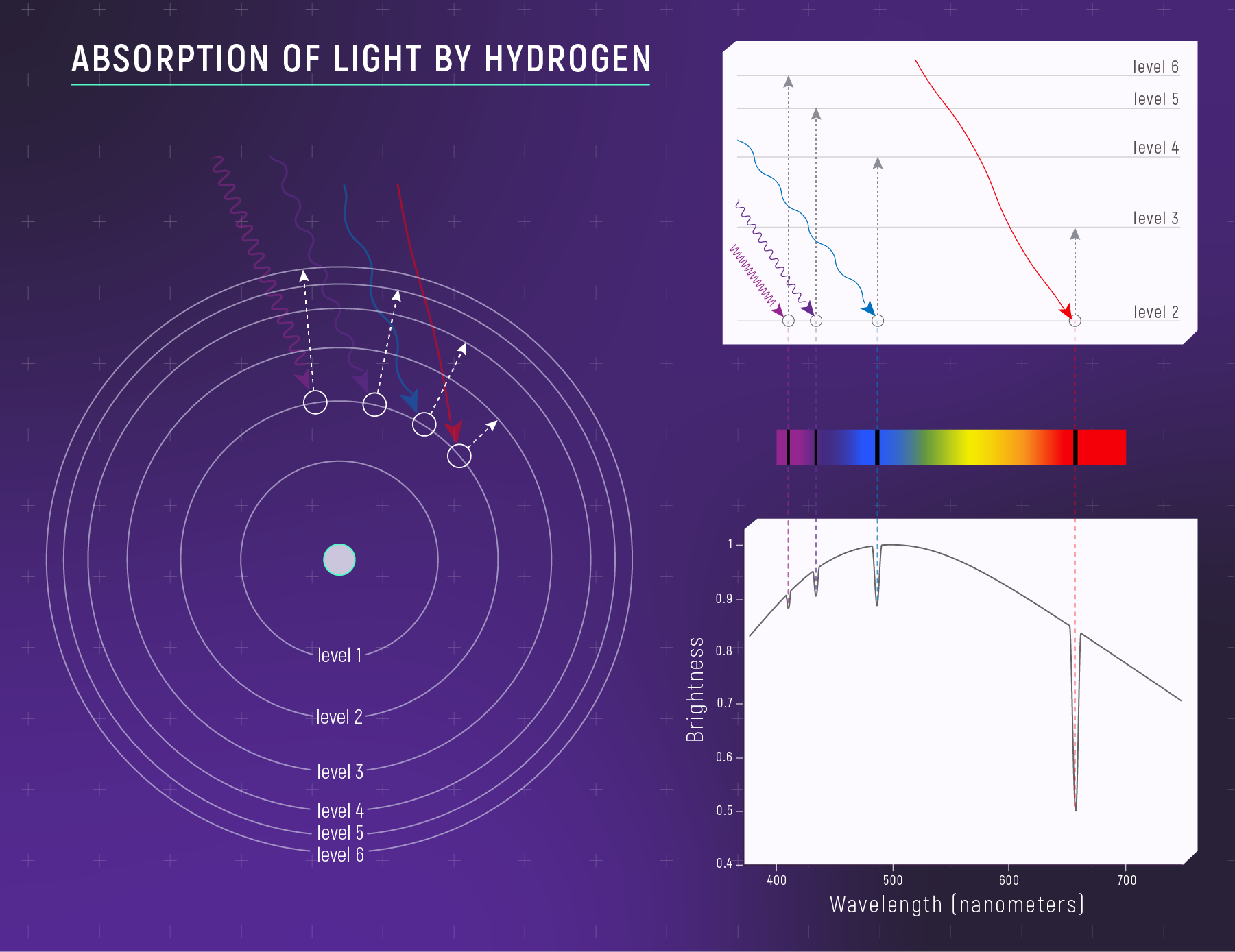
Absorption: Photon In, Electron Up

You see dark lines when:

• light passes through cooler gas
• specific photon energies are removed

Credit: JWST/STScI

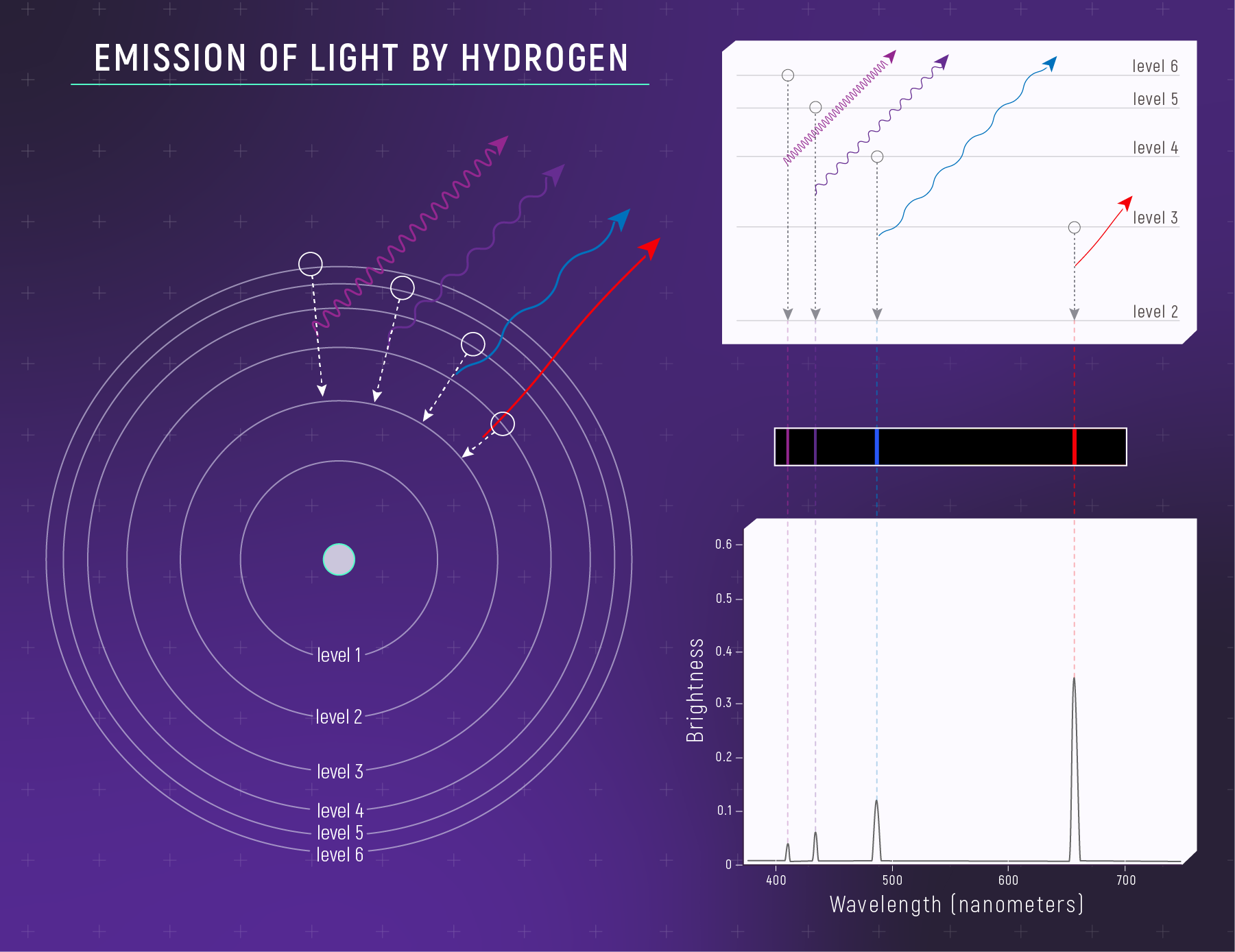
Emission: Electron Down, Photon Out

You see bright lines when:

• excited gas emits
• photons come out at specific energies

Credit: JWST/STScI

Kirchhoff’s Laws (The Three Spectrum Types)

Credit: JWST/STScI

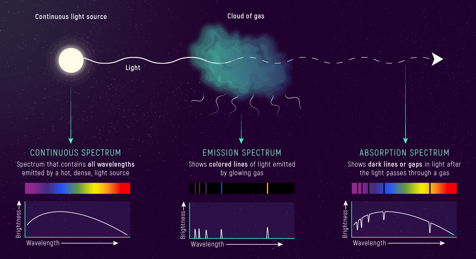
Anchor the three cases: 1) hot dense → continuous 2) continuous + cooler gas in front → absorption 3) hot thin gas → emission

Kirchhoff Summary (For Studying)

• hot, dense → continuous
• continuous + cooler gas → absorption
• hot, thin gas → emission

🧠 Quiz: Which Spectrum?

A hot dense source shines through a cooler gas cloud in front of it. You observe…

• an emission-line spectrum
• an absorption-line spectrum
• a continuous spectrum with no lines
• a spectrum that depends only on distance

Quick Check: Name the Scenario

Which situation gives an emission-line spectrum?

• a hot dense object by itself
• a hot dense object seen through cooler gas
• a hot, low-density gas cloud
• a spectrum with no wavelength information

Element Fingerprints

Credit: JWST/STScI

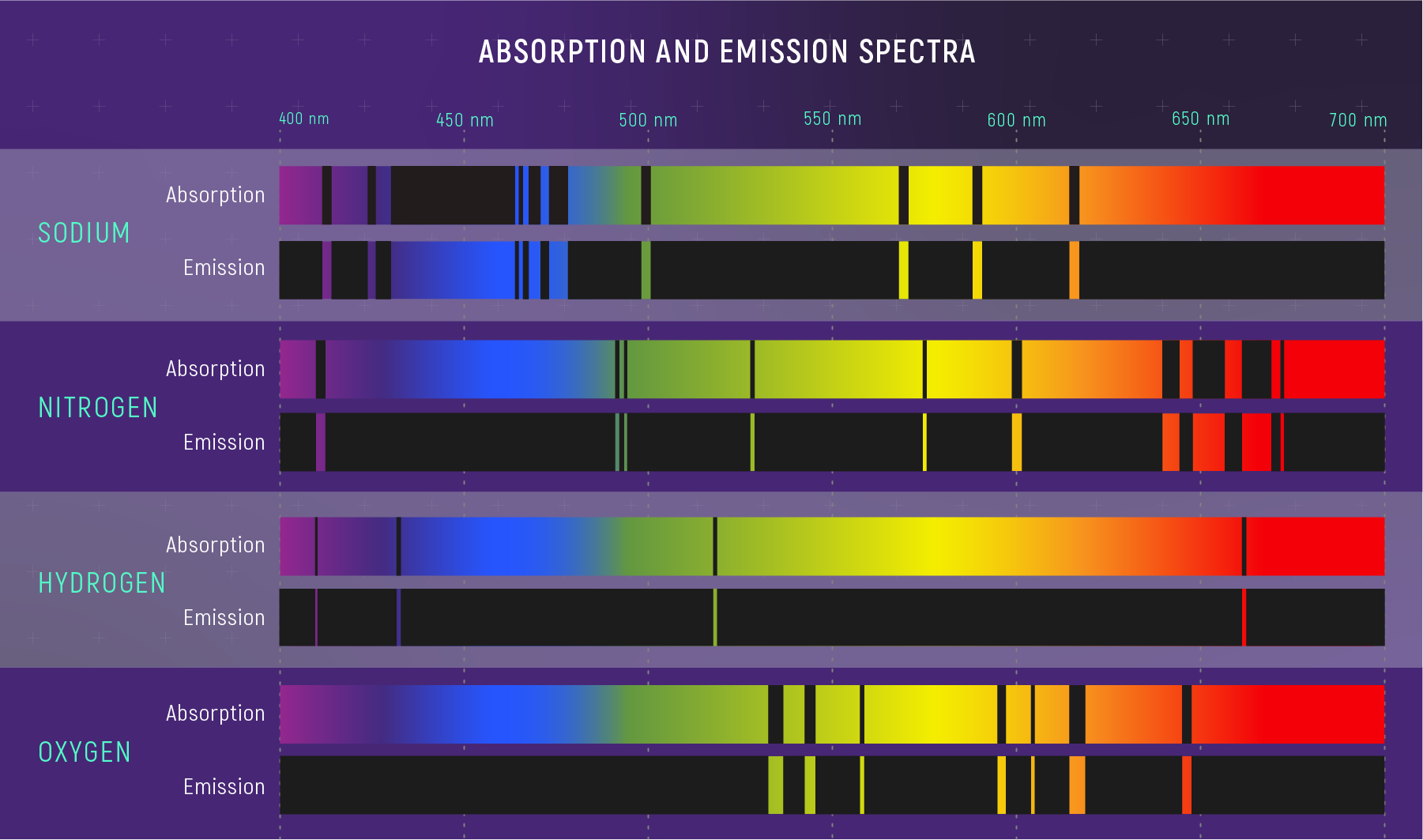
Key line: line patterns are not random — they are a fingerprint of atomic structure.

What Spectral Lines Can Tell You (Preview)

From lines alone, astronomers can infer:

• composition (which elements are present)
• temperature (which transitions are populated)
• density/pressure (line widths and ratios)
• motion (Doppler shifts — coming soon)

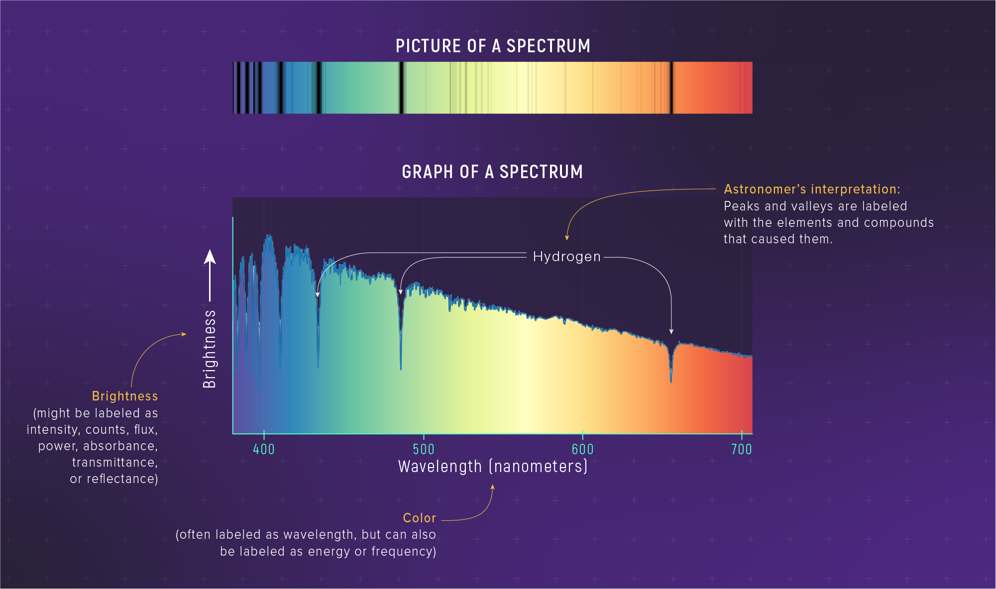
Real Stellar Spectra Combine Tools

In one observation, you can infer:

• temperature from the continuum shape
• composition from which lines appear
• (later) velocity from line shifts

Credit: JWST/STScI

Thermal vs Non-Thermal Emitters

Credit: JWST/STScI

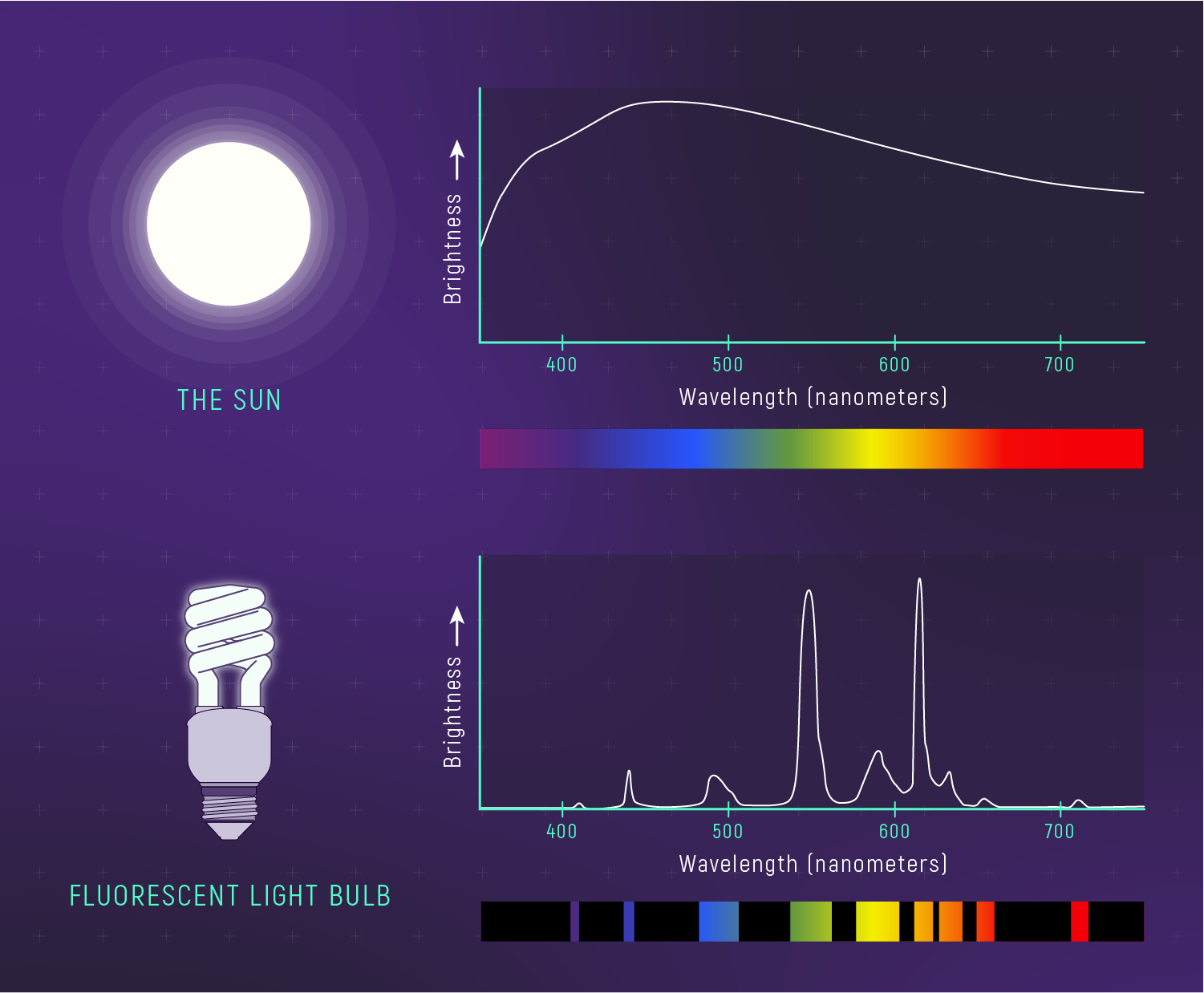
Short prompt: “Which one looks blackbody-like?” Tie back: different physics → different spectrum shapes.

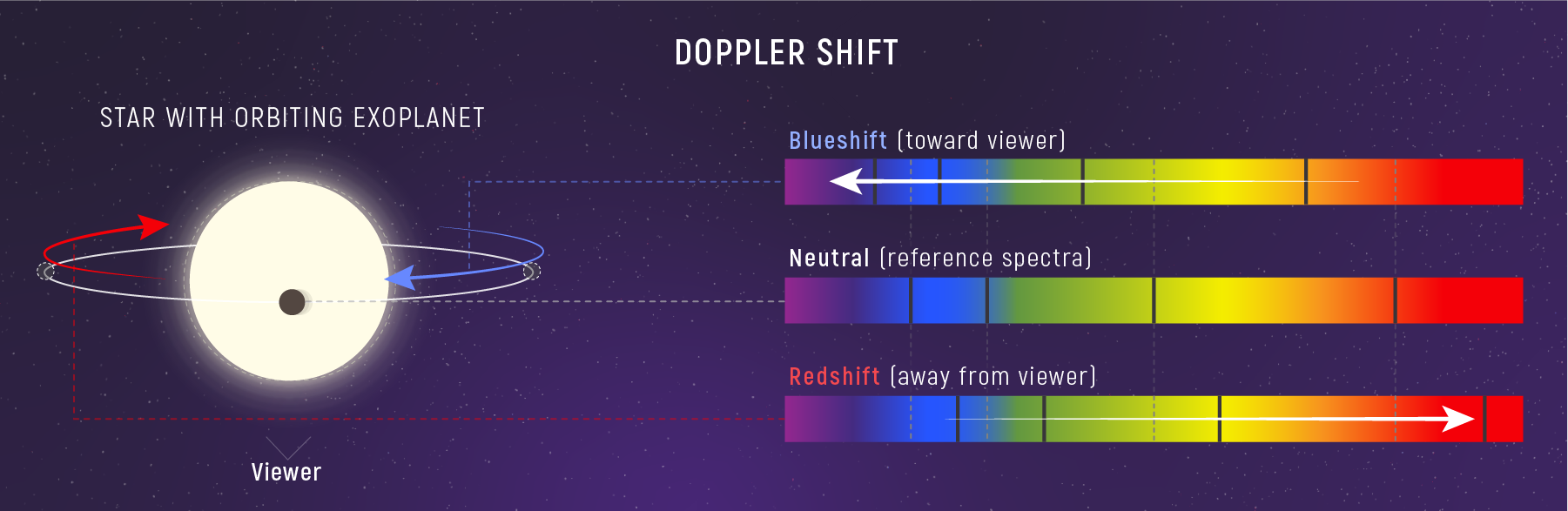
Doppler Shift = Motion from Light

Spectral lines are fixed fingerprints in the lab.
When those lines shift, we are seeing motion.

Credit: JWST/STScI

Doppler is a core tool, not just a teaser. Students should leave able to compute \(v_r\) from a line shift. Emphasize: spectral lines are the ruler; the shift is the measurement.

The Doppler Equation (Small‑Velocity Limit)

\[\frac{\Delta\lambda}{\lambda_0} = \frac{v_r}{c}\]

• \(\Delta\lambda = \lambda_{\text{obs}} - \lambda_0\) (shift from rest wavelength)
• \(v_r\) is line‑of‑sight velocity (positive = moving away)
• Assumes \(v_r \ll c\); if \(v_r = 0\), then \(\Delta\lambda = 0\)

Misconception Check: “Red” and “Blue”

Redshift does not mean “only red light.”
Blueshift does not mean “only blue light.”

• The entire spectrum shifts: every wavelength stretches or compresses.
• The names come from direction (toward red = longer \(\lambda\), toward blue = shorter \(\lambda\)), not from the color of the source.

Example: a spectral line at 500 nm shifts to 500.5 nm — still visible, just slightly longer. This is why we can measure velocities from line positions even when the object looks white.

Why This Is Powerful

Because of tiny line shifts, we can measure things we can’t touch:

• Exoplanets via stellar wobble
• Binary star masses from orbital speeds
• Galaxy rotation curves (dark matter)
• Cosmic expansion (redshift)

🧠 Quick Check: Direction

A spectral line appears at a longer wavelength than its lab value. The source is…

• moving away (redshift)
• moving toward (blueshift)
• motionless
• moving sideways only

Part 3: Telescopes Turn Light Into Inference

More photons and finer detail.

Collecting Area: Why Bigger Is Better

The number of photons you collect scales like:

\[A \propto D^2\]

Double \(D\) → 4× photons.

Credit: Illustration: A. Rosen (SVG)

Collecting Area: Quick Example

If one telescope has diameter \(D\) and another has \(2D\):

\[\frac{A_2}{A_1} = \left(\frac{2D}{D}\right)^2 = 4\]

Say: “This is why big telescopes are photon machines.”

🧠 Predict (Collecting Area)

A telescope with 3× the diameter collects how much more light?

• 3×
• 6×
• 9×
• 27×

Angular Resolution: Why Bigger Is Sharper

Diffraction sets a fundamental limit:

\[\theta \propto \lambda D^{-1}\]

• bigger \(D\) → smaller \(\theta\) (sharper)
• longer \(\lambda\) → larger \(\theta\) (blurrier)

Credit: Illustration: A. Rosen (SVG)

Misconception Check: Magnification vs Resolution

More magnification does not create more detail if the image is already blurred.

Resolution is set by \(D\) and \(\lambda\) (and the atmosphere), not the zoom knob.

Quick live example: “Zooming a blurry photo doesn’t add pixels.”

The Rayleigh Criterion (Name the Rule)

For a circular aperture, the diffraction limit is approximately:

\[\theta \approx 1.22\,\lambda D^{-1}\]

You can mention “1.22 is geometry” and the scaling is the important part.

🧠 Predict (Resolution)

Same telescope, same target. Switching from visible to infrared (longer \(\lambda\)) makes resolution…

• better
• worse
• unchanged
• dependent only on magnification

Instruments + Atmosphere

Two reasons we build space telescopes:

• blocked wavelengths (no ground X-ray astronomy)
• atmospheric blurring (seeing)

Credit: NASA

Mirrors vs Lenses (Brief)

Why big telescopes are mirrors:

• lenses absorb/warp light when they get large
• mirrors can be supported from behind
• reflective coatings can work across many wavelengths

Keep it short. This is “engineering constraints shape what we can measure.”

Synthesis (Day 2)

We now have a powerful inference chain:

• continuum → temperature (blackbody + Wien)
• lines → composition (and motion)
• telescopes → more photons + better detail

Everything we do next semester-wide is built on this.

Demo Time (If Time): Telescope Resolution

Demo: telescope-resolution

Prompt: What matters more for resolution — aperture or magnification? What does wavelength do?

Local path (instructor): /Users/anna/Teaching/astr101-sp26/demos/telescope-resolution/ Suggested flow (5–8 min): 1) Start with “binary star” view; ask students to predict resolved/unresolved. 2) Increase D at fixed λ: show the Airy disk shrinking. 3) Increase λ at fixed D: show resolution getting worse. If you’re short on time: do only step (1) + one slider move.

Exit Ticket (30 seconds)

Pick one:

1. “One new inference we can make from spectra is…”
2. “One reason we build big telescopes is…”

Collect 2–3 aloud. Listen for continuum vs lines distinction.

Study Snapshot (Write This Down)

• continuum → \(T\) (blackbody + Wien)
• lines → composition
• \(A\propto D^2\) (photons)
• \(\theta\propto \lambda D^{-1}\) (detail)

This is the “what to memorize” compression slide.