flowchart LR
  O["🔭 Observable\nWhat we measure"]
  M["📐 Model\nWhat we assume"]
  I["💡 Inference\nWhat we derive"]
  O --> M --> I
  style O fill:#dbeafe,stroke:#2563eb
  style M fill:#fef3c7,stroke:#d97706
  style I fill:#dcfce7,stroke:#16a34a
Lecture 1: Distance & Parallax
How far? The foundation of stellar astrophysics
Parallax, the inverse-square law, and the measurement chain from angular shift to luminosity.
Learning Objectives
By the end of this lecture, you will be able to:
- Define angular measure (degrees, arcminutes, arcseconds, radians) and convert between them
- Derive and apply the small-angle approximation to relate angular size, true size, and distance
- Define parallax angle and the parsec; calculate distances from parallax measurements
- Derive the inverse-square law (geometric + dimensional analysis approaches)
- Apply \(F = L/(4\pi d^2)\) to infer luminosity from flux and parallax distance
Read these aloud. Students should write them down or note them. Estimated time: 1–2 min.
Are all stars like our Sun?
0–1 min. Let this sit for 5 seconds. Build curiosity before explaining. This is the hook — the answer is no, but we don’t know that yet just by looking at the sky.
The Problem: Points of Light

Credit: cococubed.com
1–2 min. Point to the figure: stars appear projected onto one sphere, but they’re actually at wildly different distances. A faint dot could be a nearby red dwarf or a distant blue supergiant.
Quick Check 1: Are Stars Like Our Sun?
Two stars appear equally bright in your telescope. What can you conclude?
A. They have the same luminosity
B. They are at the same distance
C. You can’t tell — brightness depends on both luminosity and distance
D. The brighter-looking one must be closer
2–3 min. Give students 30 seconds. Use iClicker. Answer: C. This is the fundamental degeneracy. Equal apparent brightness tells you nothing about intrinsic properties without knowing distance.
The Degeneracy Problem
Equal apparent brightness can mean:
Scenario 1: A luminous star far away
\[F = \frac{L_{\text{high}}}{4\pi d_{\text{far}}^2}\]
Scenario 2: A dim star nearby
\[F = \frac{L_{\text{low}}}{4\pi d_{\text{near}}^2}\]
The same flux \(F\) — completely different stars. Without distance, you’re stuck.
3–4 min. This motivates the entire lecture: distance breaks the degeneracy.
Distance Is the Master Key
\[\text{Parallax} \xrightarrow{d = 1/p} \text{Distance} \xrightarrow{d + F} \text{Luminosity} \xrightarrow{L + T} \text{HR Diagram}\]
- Distance + apparent brightness = luminosity (today)
- Luminosity + temperature = radius (Lecture 2)
- Distance + spectrum = composition (Lecture 3)
- Distance + radial velocity = mass (Lecture 4)
Everything starts with distance.
4–5 min. This is the roadmap for Module 2. Today we solve the first link in the chain.
The Observable → Model → Inference Framework
| Step | This lecture |
|---|---|
| Observable | Position shifts, brightness |
| Model | Parallax geometry, ISL |
| Inference | Distance, luminosity |
Good scientists always ask: what am I assuming, and what would break it?
5–6 min. This framework appears in every lecture. Establish it clearly here. The Mermaid diagram makes the flow visual — point to each box.
Angular Measure
The language of the sky
Degrees, Arcminutes, Arcseconds
| Unit | Size |
|---|---|
| \(1^\circ\) | Full Moon width |
| \(1'\) (arcmin) | \(1/60\) of a degree |
| \(1''\) (arcsec) | \(1/3600\) of a degree |

Credit: cococubed.com
Stellar parallax happens at the arcsecond scale — tiny shifts against distant background stars.
7–8 min. Emphasize: arcseconds are angles, not distances. A common misconception.
Radians — The Natural Unit
Definition: 1 radian is the angle subtended by an arc whose length equals the radius.
\[1 \text{ radian} = \frac{360^\circ}{2\pi} \approx 57.3^\circ\]
Radians are dimensionless: angle = arc length / radius = length / length.

Credit: cococubed.com
Physics formulas like \(\sin\theta \approx \theta\) and \(v = r\omega\) only work in radians.
8–9 min. Key point: radians make the math clean. The small-angle approximation requires radians.
The Key Conversion: Arcseconds ↔︎ Radians
\[1 \text{ radian} = \frac{360 \times 3600''}{2\pi} \approx 206{,}265''\]
Inverted (the form you’ll use most):
\[\boxed{1'' = \frac{1}{206{,}265} \text{ rad} \approx 4.85 \times 10^{-6} \text{ rad}}\]
Memorize 206,265. It appears in every parallax calculation.
9–10 min. This number bridges the two systems. Quick-check: \(2 \times 10^5\) for mental math.
The Small-Angle Approximation
Connecting angular size, true size, and distance
The Geometric Picture
For small angles (\(\alpha \ll 1\) rad):
\[\boxed{\alpha\,(\text{rad}) \approx \frac{s}{d}}\]
- \(\alpha\) = angular size (radians)
- \(s\) = true (physical) size
- \(d\) = distance to object
Physical meaning: Angular size is inversely proportional to distance.
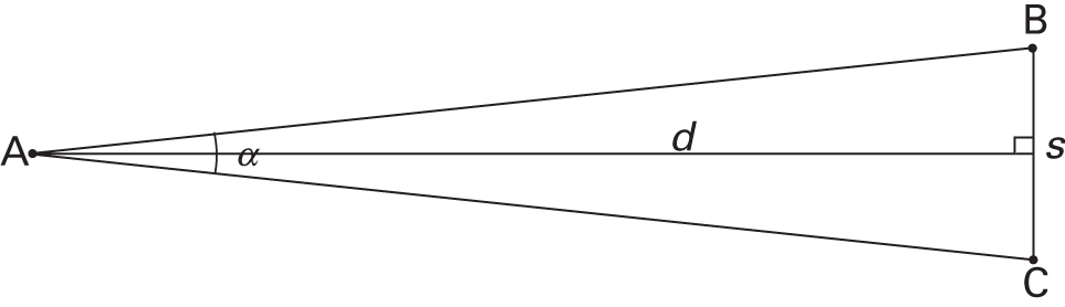
Credit: Fundamentals of Astrophysics (Owocki)
11–12 min. Walk through the geometry: arc length ≈ chord length for small angles. Both \(s\) and \(d\) must be in the same units.
Why Does It Work? sin θ ≈ θ
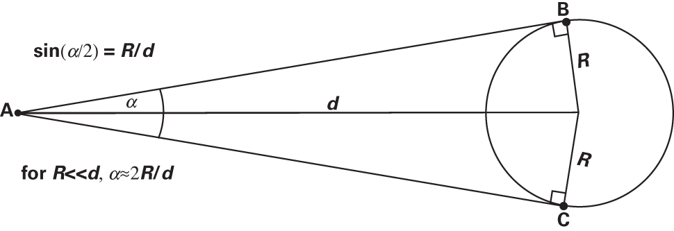
Credit: Fundamentals of Astrophysics (Owocki)
The exact relation: \(\sin(\alpha/2) = R/d\)
For small \(\alpha\): \(\sin(\alpha/2) \approx \alpha/2\)
\[\implies \alpha \approx \frac{2R}{d} = \frac{s}{d}\]
How small is “small enough”?
At \(\alpha = 5°\), error is only 0.1%. For astronomy (arcseconds!), it’s essentially exact.
12–13 min. This figure shows the exact vs approximate relation. The takeaway: for any angle smaller than a few degrees, the approximation is superb.
Quick Check 2: Small-Angle Scaling
If you double your distance from an object (keeping its true size fixed), its angular size:
A. Doubles
B. Quadruples
C. Halves
D. Quarters
12–13 min. Give students 30 seconds. Use iClicker. Answer: C. Since \(\alpha \approx s/d\), doubling \(d\) halves \(\alpha\). This is linear, not quadratic — angular size scales as \(1/d\), not \(1/d^2\).
Worked Example: Moon’s Diameter
Given:
- Angular size: \(\alpha = 0.5^\circ\)
- Distance: \(d = 3.84 \times 10^{10}\) cm
Convert: \(0.5^\circ = 1800'' \div 206{,}265 = 0.00873\) rad
Apply: \(s = \alpha \, d\)
\[s = (0.00873)(3.84 \times 10^{10} \text{ cm})\] \[\approx 3{,}350 \text{ km}\]
Actual lunar diameter: 3,474 km
Agreement within 4% — excellent!
. . .
The small-angle approximation works beautifully at half-degree scales.
13–14 min. Walk through units carefully: radians are dimensionless, so \(s\) inherits the units of \(d\).
Parallax
Distance from baseline geometry
Try It First: Parallax Demo
Before we derive anything, explore the interactive demo:
- Move the star closer and farther — watch the parallax angle change
- Closer star → larger parallax shift; the shift is measured against distant background stars
Now let’s derive why this works. → Full-screen demo
15–16 min. The demo is embedded — interact with it live. If the embed doesn’t load, click the full-screen link. Give students 60 seconds to explore.
Parallax: The Geometry
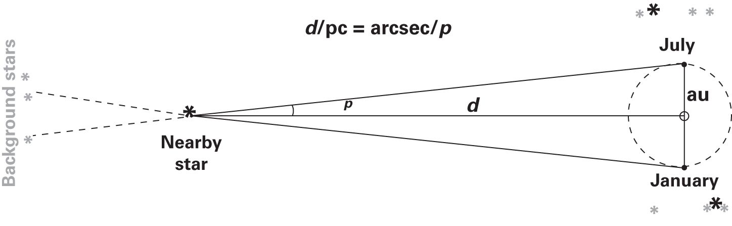
As Earth orbits, a nearby star appears to shift against distant background stars.
The parallax angle \(p\) is defined as half the total shift, using a baseline of 1 AU (Earth’s orbital radius).
\[p\,(\text{rad}) \approx \frac{1\,\text{AU}}{d}\]

Credit: cococubed.com
16–17 min. Point to the figure: identify the baseline (1 AU), the parallax angle \(p\) (at the star), and the distance \(d\).
From Geometry to the Parsec
Convert parallax to arcseconds:
\[p\,('') = \frac{1\,\text{AU}}{d} \times 206{,}265\]
Define: 1 parsec (pc) = distance at which \(p = 1''\)
\[1\,\text{pc} = 206{,}265\,\text{AU} = 3.09 \times 10^{18}\,\text{cm} = 3.26\,\text{ly}\]
The distance formula becomes breathtakingly simple:
\[\boxed{d\,(\text{pc}) = \frac{1}{p\,('')}}\]
Credit: Fundamentals of Astrophysics (Owocki)
17–18 min. “Parsec” = parallax arcsecond. The unit is defined to make the formula simple — it bakes in Earth’s orbital radius. Point to the figure: 1 AU baseline, parallax angle \(p\), distance \(d\).
Quick Check 3: Parallax and Distance
Star A has parallax \(p = 0.5''\). Star B has parallax \(p = 0.1''\).
A. Star A is closer (2 pc vs 10 pc)
B. Star B is closer (10 pc vs 2 pc)
C. They’re at the same distance
D. Can’t tell without knowing luminosity
18–19 min. Give students 30 seconds. Answer: A. \(d = 1/p\), so larger parallax → shorter distance. Star A is at 2 pc, Star B at 10 pc.
Worked Example: Proxima Centauri
Given: \(p = 0.768''\) (nearest star)
Step 1: Distance in parsecs \[d = \frac{1}{0.768} = 1.30\,\text{pc}\]
Step 2: Convert to centimeters \[d = 1.30 \times 3.09 \times 10^{18}\,\text{cm pc}^{-1}\] \[= 4.02 \times 10^{18}\,\text{cm}\]
Sanity check:
Nearby stars should be 1–5 pc. ✓
. . .
At 1.3 pc, Proxima is \(\sim 25\) trillion miles away — yet it’s the closest star.
This shows why parallax was historically so difficult to measure.
19–20 min. Emphasize the sanity check step — students should always verify their answers are physically reasonable.
Our Nearest Neighbors

Credit: cococubed.com
The nearest stellar neighborhood is a sparse place.
- Proxima Centauri: 1.3 pc
- Sirius: 2.6 pc
- Within 5 pc: only \(\sim 60\) known stellar systems
Most are red dwarfs too faint to see with the naked eye — the night sky is biased toward luminous stars.
20–21 min. This 3D map shows distances measured by parallax. Point out how few stars are truly nearby. Connect to the degeneracy problem: apparent brightness ≠ nearness.
The Parallax Revolution: Hipparcos to Gaia
| Mission | Precision | Stars | Distance reach |
|---|---|---|---|
| Ground (pre-1990) | \(\sim 50\) mas | \(\sim 1{,}000\) | \(\sim 20\) pc |
| Hipparcos (1989–93) | \(\sim 1\) mas | \(\sim 100{,}000\) | \(\sim 100\) pc |
| Gaia (2013–25) | \(\sim 10\) \(\mu\)as | \(\sim 1.8\) billion | \(\sim 10\) kpc |
Gaia’s \(100\times\) better precision directly translates to \(100\times\) better luminosity measurements for every star observed.
20–21 min. Gaia completed science observations January 2025; Data Release 4 expected late 2026. This mission has reshaped all of stellar astrophysics.
Active Learning Break 1: Think-Pair-Share
Problem: A star has parallax \(p = 0.050''\).
(a) What is its distance in parsecs?
(b) Convert to light-years.
(c) Could Hipparcos have measured this parallax? Could Gaia?
(d) Estimate the parallax of a star at the center of the Milky Way (\(\sim 8\) kpc away).
Credit: cococubed.com
Reference: parallax geometry
Answers: (a) \(d = 1/0.050 = 20\) pc. (b) \(20 \times 3.26 = 65\) ly. (c) Yes (Hipparcos limit \(\sim 1\) mas \(= 0.001''\), this is much larger). (d) \(p = 1/8000 = 0.000125'' = 125\,\mu\)as — detectable by Gaia.
21–25 min (4 min total). 90 seconds silent work. 90 seconds pair discussion. 1 minute share. Cold-call for part (d).
The Inverse-Square Law
How light spreads through space
Predict First
If you move twice as far from a light source, by what factor does the brightness change?
Think about why before we derive it.
25–26 min. Give 15 seconds of silent think time. Don’t reveal yet — let them commit to an answer.
Geometric Derivation: Concentric Spheres
A star emits luminosity \(L\) uniformly in all directions.
At distance \(d\), this energy is spread over a sphere of area \(4\pi d^2\).
Flux = energy per time per area:
\[\boxed{F = \frac{L}{4\pi d^2}}\]

Credit: Course illustration (A. Rosen)
Double the distance → flux drops by 4×. Ten times farther → flux drops by 100×.
26–28 min. Walk through the geometry. The \(4\pi\) comes from the full solid angle of a sphere. Point to the figure: same total energy, larger sphere, less per unit area.
Quick Check 4: Inverse-Square Law
You move 3× farther from a lamp. By what factor does the brightness drop?
A. 3× dimmer
B. 6× dimmer
C. 9× dimmer
D. 27× dimmer
28–29 min. Give students 30 seconds. Use iClicker. Answer: C. \(F \propto 1/d^2\), so \(3^2 = 9\). Common error: choosing A (linear thinking) or D (cubic thinking).
Dimensional Analysis Check
Assume \(F \propto L^a \, d^b\)
| Quantity | Dimension |
|---|---|
| \(F\) (flux) | \([M\,T^{-3}]\) |
| \(L\) (luminosity) | \([M\,L^2\,T^{-3}]\) |
| \(d\) (distance) | \([L]\) |
Match exponents:
- Mass: \(1 = a\) → \(a = 1\)
- Time: \(-3 = -3a\) ✓
- Length: \(0 = 2a + b\) → \(b = -2\)
\[F \propto \frac{L}{d^2}\]
The \(4\pi\) comes from geometry — DA gives the scaling.
29–30 min. Two independent derivations → same answer. This convergence builds confidence. Reference Module 1 Lecture 2 tools.
Where Does the 4π Come From?
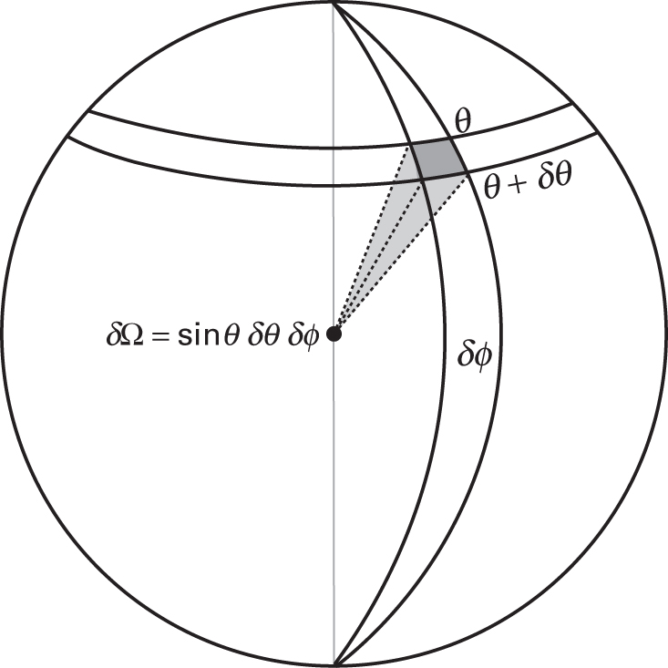
Credit: Fundamentals of Astrophysics (Owocki)
A full sphere subtends \(4\pi\) steradians of solid angle.
Light from an isotropic source spreads evenly over this solid angle. At distance \(d\), the sphere has area \(4\pi d^2\).
So \(F = L/(4\pi d^2)\) simply says: total luminosity ÷ total area of the sphere you’re standing on.
30–31 min. This figure connects the \(4\pi\) factor to geometry. The solid angle concept is introduced here and returns in surface brightness (Module 2 Lecture 2).
Flux vs. Luminosity — Don’t Confuse Them!
Flux \(F\) (what you measure)
- Depends on where you stand
- Units: erg cm\(^{-2}\) s\(^{-1}\)
- Changes with distance
Luminosity \(L\) (what the star emits)
- Intrinsic property of the star
- Units: erg s\(^{-1}\)
- Does not depend on distance
A dim red dwarf nearby can have the same observed flux as a luminous blue giant far away. You cannot determine luminosity from flux alone — you always need distance.
31–32 min. This is the single most important conceptual point. Hammer it home.
A Useful Surprise: Surface Brightness Is Distance-Independent
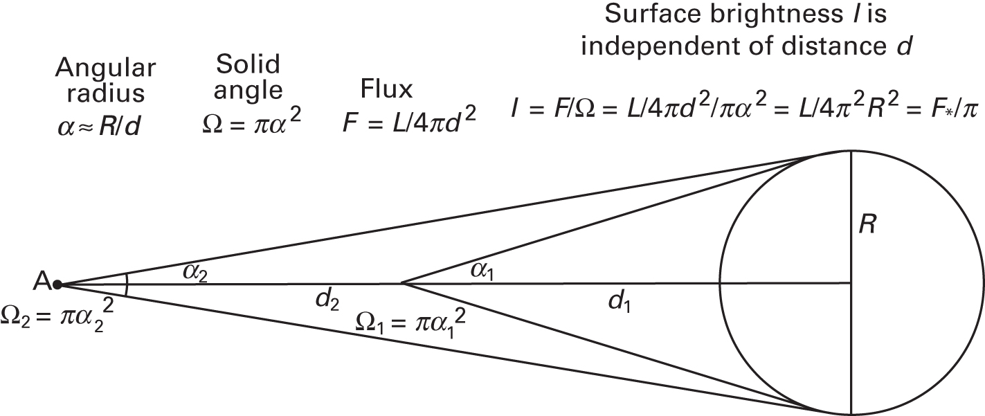
Credit: Fundamentals of Astrophysics (Owocki)
Flux drops as \(1/d^2\), but angular area also drops as \(1/d^2\).
Their ratio — surface brightness — is constant:
\[\frac{F}{\Delta\Omega} = \frac{L/(4\pi d^2)}{\pi R^2/d^2} = \frac{L}{4\pi^2 R^2}\]
This is why galaxy images don’t “fade” at greater distances — they just get smaller. Surface brightness depends only on the source, not distance.
32–33 min. This is a beautiful consequence of the ISL. It surprises students: “I thought everything gets dimmer!” — it does, but so does the apparent area. We’ll use this in Lecture 2.
From Distance to Luminosity
The measurement chain
The Complete Measurement Chain
- Observe position shifts → parallax \(p\)
- Model parallax geometry → distance \(d = 1/p\)
- Observe brightness → flux \(F\)
- Model inverse-square law → \(L = 4\pi d^2 F\)
- Infer luminosity \(L\)
Three rearrangements of one equation:
| Know | Find | Formula |
|---|---|---|
| \(L, d\) | \(F\) | \(F = L/(4\pi d^2)\) |
| \(F, d\) | \(L\) | \(L = 4\pi d^2 F\) |
| \(L, F\) | \(d\) | \(d = \sqrt{L/(4\pi F)}\) |
32–33 min. Form 2 builds the HR diagram. Form 3 is for standard candles (Part 7 of reading).
Worked Example: Solar Luminosity
Given:
- Solar constant: \(F_\odot = 1.4 \times 10^6\) erg cm\(^{-2}\) s\(^{-1}\)
- Earth–Sun distance: \(d = 1.5 \times 10^{13}\) cm
Calculate:
\[L_\odot = 4\pi d^2 F\] \[= 4\pi (1.5 \times 10^{13})^2 (1.4 \times 10^6)\] \[= 4\pi \times 3.15 \times 10^{32}\] \[\approx 3.96 \times 10^{33}\,\text{erg s}^{-1}\]
Credit: Course illustration (A. Rosen)
Standard value: \(L_\odot = 3.83 \times 10^{33}\) erg s\(^{-1}\)
Agreement within 4%!
This is how we know the Sun’s luminosity. Every star on the HR diagram uses this same method.
33–35 min. Walk through units: cm² cancels cm⁻², leaving erg s⁻¹. Emphasize that this exact method applies to every star.
Error Propagation: Why Precision Matters
\[d = \frac{1}{p} \implies \frac{\delta d}{d} \approx \frac{\delta p}{p}\]
\[L = 4\pi d^2 F \implies \frac{\delta L}{L} \approx 2\,\frac{\delta d}{d}\]
The complete chain:
10% parallax error → \(\sim 10\)% distance error → \(\sim\)20% luminosity error
Errors double going from distance to luminosity because \(L \propto d^2\).
Gaia’s \(100\times\) parallax improvement → \(100\times\) better luminosity.
35–37 min. This is why Gaia was worth building. Parallax precision cascades through the entire measurement chain.
Worked Example: Full Chain — Parallax to Astrophysics
Given: \(p = 0.214''\), \(F = 1.1 \times 10^{-7}\) erg cm\(^{-2}\) s\(^{-1}\)
Step 1: \(d = 1/0.214 = 4.67\) pc \(= 1.44 \times 10^{19}\) cm
Step 2: \[L = 4\pi (1.44 \times 10^{19})^2 (1.1 \times 10^{-7})\] \[\approx 2.9 \times 10^{32}\,\text{erg s}^{-1}\]
Step 3: \(L/L_\odot = 2.9 \times 10^{32} / 3.83 \times 10^{33} \approx 0.075\)
Credit: ESO
This star at \(L \approx 0.08\,L_\odot\) sits on the lower main sequence — a late K or early M dwarf. These small, cool, red stars dominate the Galaxy by number.
37–39 min. This is the full pipeline in action. A tiny angular shift + a brightness measurement reveals the fundamental nature of a star.
Active Learning Break 2: Synthesis Problem
A star has parallax \(p = 0.1''\) and flux \(F = 10^{-11}\) erg cm\(^{-2}\) s\(^{-1}\).
- Distance? (\(d = 10\) pc \(= 3.09 \times 10^{19}\) cm)
- Luminosity? (\(L = 4\pi d^2 F \approx 1.2 \times 10^{29}\) erg s\(^{-1}\))
- In solar luminosities? (\(L/L_\odot \approx 3 \times 10^{-5}\))
- What kind of star? (Very faint red dwarf — \(\sim 30{,}000\times\) dimmer than the Sun!)
Credit: ESO
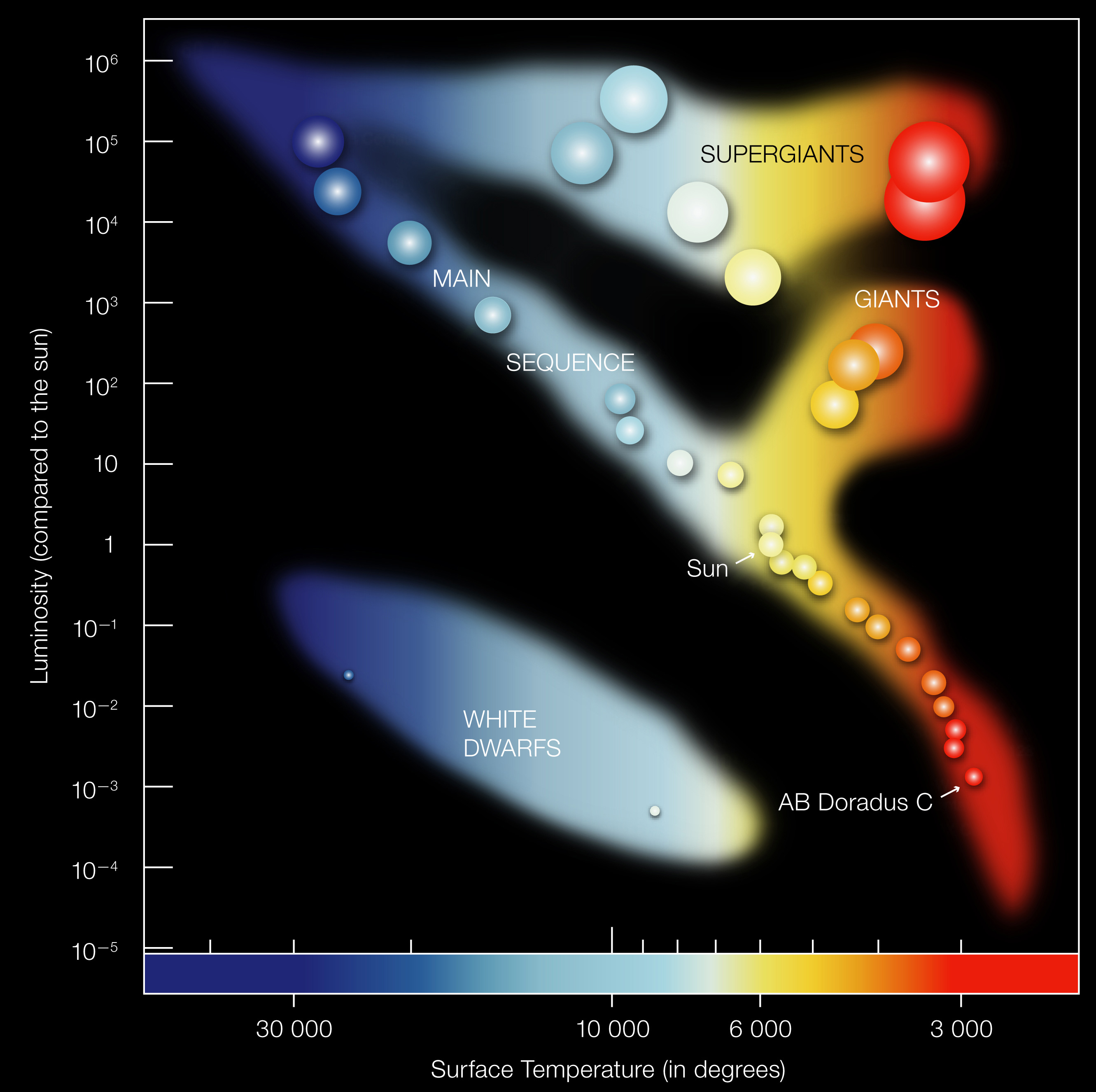
Where does your answer land on the HR diagram?
39–42 min (3 min total). 90 seconds individual work. 90 seconds pair discussion. Quick poll: “Who got something in the range \(10^{28}\)–\(10^{30}\)?” Point to the HR diagram — their star sits at the very bottom of the main sequence.
Quick Check 5: Putting It Together
Two stars have identical flux. Star A is at 10 pc, Star B at 100 pc. Which has higher luminosity, and by what factor?
A. Star A, by 10×
B. Star B, by 10×
C. Star A, by 100×
D. Star B, by 100×
42–43 min. Give students 30 seconds. Use iClicker. Answer: D. Since \(L = 4\pi d^2 F\) and \(F\) is the same, \(L \propto d^2\). Star B is 10× farther, so \(L_B/L_A = (100/10)^2 = 100\). Star B is 100× more luminous.
Beyond Parallax
Standard candles and the distance ladder
The Parallax Horizon
Parallax works out to:
- \(\sim 100\) pc from ground-based telescopes
- \(\sim 10\) kpc with Gaia
But the Milky Way is \(\sim 30\) kpc across, and Andromeda is \(\sim 770\) kpc away.
How do we measure distances beyond parallax?
44–45 min. Set up the need for standard candles.
Standard Candles: Using the ISL Backwards
If we know a star’s luminosity \(L\), we can measure its flux \(F\) and infer distance:
\[\boxed{d = \sqrt{\frac{L}{4\pi F}}}\]
Objects with known or determinable luminosity are called standard candles.
Credit: Course illustration (A. Rosen)
45–46 min. The inverse-square law runs both directions: forward (flux from luminosity + distance) and backward (distance from luminosity + flux).
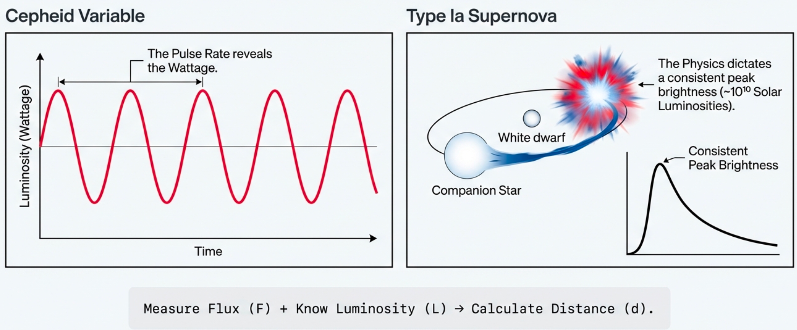
Cepheids and Type Ia Supernovae
Cepheid Variables
- Pulsating stars; period → luminosity
- Discovered by Henrietta Leavitt (1912)
- Reach: \(\sim 30\) Mpc
- Hubble used them to prove Andromeda is a separate galaxy (1920s)
Type Ia Supernovae
- Thermonuclear explosions of white dwarfs
- Peak luminosity: ~few \(\times 10^9 L_\odot\)
- Reach: \(\sim 10\) Gpc (cosmological!)
- Led to the discovery of dark energy (2011 Nobel Prize)

Credit: cococubed.com
Massive, luminous stars are rare and distant — we need long-reach methods to study them. Standard candles solve this.
46–48 min. Each standard candle extends the distance reach by orders of magnitude.
The Cosmic Distance Ladder
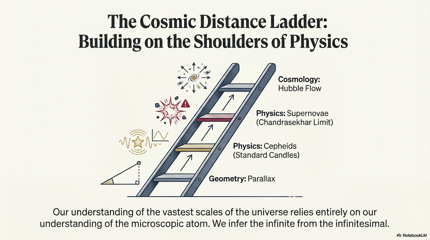
Credit: Course illustration (A. Rosen)
Each rung is calibrated by the one below. The entire cosmic distance scale rests on getting nearby parallaxes right — which is why Gaia matters for all of astronomy.
48–50 min. Parallax → Cepheids → Type Ia supernovae. When Gaia improved nearby parallaxes, it rippled through the entire ladder. Point to each rung in the figure.
Wrapping Up
Summary: Key Equations
| Equation | What it does |
|---|---|
| \(\alpha \approx s/d\) | Angular size ↔︎ true size + distance |
| \(d\,(\text{pc}) = 1/p\,('')\) | Parallax → distance |
| \(F = L/(4\pi d^2)\) | Inverse-square law |
| \(L = 4\pi d^2 F\) | Luminosity from flux + distance |
| \(d = \sqrt{L/(4\pi F)}\) | Standard candle distance |
Credit: cococubed.com
flowchart LR
  P["Position shift\n(Observable)"] --> G["Parallax geometry\n(Model)"]
  G --> D["Distance d\n(Inference)"]
  F["Flux F\n(Observable)"] --> ISL["Inverse-square law\n(Model)"]
  D --> ISL
  ISL --> L["Luminosity L\n(Inference)"]
  L --> HR["HR Diagram"]
  style P fill:#dbeafe,stroke:#2563eb
  style F fill:#dbeafe,stroke:#2563eb
  style G fill:#fef3c7,stroke:#d97706
  style ISL fill:#fef3c7,stroke:#d97706
  style D fill:#dcfce7,stroke:#16a34a
  style L fill:#dcfce7,stroke:#16a34a
  style HR fill:#f3e8ff,stroke:#9333ea
50–52 min. The Mermaid diagram is the complete measurement chain. Blue = observables, yellow = models, green = inferences, purple = destination. Point to each node.
The Takeaway
If you forget everything else from today, remember this:
Distance is the master key.
Measure distance, and luminosity becomes knowable — the first step to understanding any star.
52–53 min. This is the core message. Make it memorable.
Questions?
Common questions at this point:
- “Why can’t we just use radar to measure star distances?”
- “What if dust absorbs the light — doesn’t that break the inverse-square law?”
- “How do we know the period-luminosity relation for Cepheids is correct?”
53–55 min. Address these directly. Radar: only works for solar system objects (light-travel time too long for stars). Dust: yes, extinction corrections are essential. Cepheids: calibrated using nearby Cepheids with parallax distances — the ladder at work.
Looking Ahead
Next time (Lecture 2): Surface Flux & Colors of Stars
- Stefan-Boltzmann law: \(L = 4\pi R^2 \sigma T^4\)
- Wien’s law: peak wavelength → temperature
- Stellar radii from luminosity + temperature
Before then:
- Read: Lecture 1 reading (distance & parallax)
- Try: Practice problems 3–5 (parallax conversions & luminosity calculations)
55–57 min. Connect to what’s coming. Lecture 2 adds the second axis of the HR diagram (temperature).
Equation Toolbox — Your Reference Card
| Equation | Form | When to use |
|---|---|---|
| Angle conversions | \(1^\circ = 3600''\); \(1' = 60''\) | Angular unit conversion |
| Arcsec ↔︎ radians | \(1\,\text{rad} = 206{,}265''\) | Bridging measurement systems |
| Small-angle | \(\alpha\,(\text{rad}) \approx s/d\) | Angular size, true size, distance |
| Parallax–distance | \(d\,(\text{pc}) = 1/p\,('')\) | Parallax to distance |
| Inverse-square law | \(F = L/(4\pi d^2)\) | Flux, luminosity, distance |
| Luminosity inference | \(L = 4\pi d^2 F\) | Computing luminosity |
| Standard candle | \(d = \sqrt{L/(4\pi F)}\) | Distance from known luminosity |
Reference slide for students to photograph or bookmark. Not meant to be presented — just available.