Lecture 2: Surface Flux and Colors

From color to temperature to radius

Dr. Anna Rosen

February 12, 2026

Today’s Targets (What you should be able to do after class)

By the end of Lecture 2, you can:

• Distinguish received flux \(F\) from surface flux \(F_\star\) (they answer different questions).
• Use Stefan-Boltzmann to connect \(L\), \(R\), \(T\) and do scaling quickly.
• Use Wien’s law to infer \(T\) from \(\lambda_{\rm peak}\) (especially with ratios).
• Explain (briefly, correctly) the ultraviolet catastrophe and why Planck mattered.
• Read the HR diagram as a radius map in disguise (preview).

This is an inference-chain lecture. The equations are tools, not the point.

The Big Idea

Astronomy is an inference machine.

We measure photons at Earth (brightness + spectrum) and infer physical properties of stars:

• \(F\) + \(d\) \(\rightarrow\) \(L\) (Lecture 1)
• color / \(\lambda_{\rm peak}\) \(\rightarrow\) \(T\) (today)
• \(L\) and \(T\) \(\rightarrow\) \(R\) (today)

Two observables + one distance gives you a lot of reality.

Orion Puzzle: Same Luminosity, Wildly Different Size

Rigel (blue) and Betelgeuse (red) can have comparable luminosities yet very different radii.

• Blue star: hotter \(\rightarrow\) can be smaller and still luminous
• Red star: cooler \(\rightarrow\) must be huge to be equally luminous

Warning

Same luminosity does not imply same radius. “Bright” is ambiguous — always say which quantity you mean.

I want your gut prediction before I give you the lever.

Commit to a Prediction

If two stars have the same luminosity and one is cooler, that cooler star is most likely:

• smaller
• larger
• at the same radius
• impossible to determine from physics

Don’t overthink: we’re holding \(L\) fixed. We’ll prove it.

Vocabulary Lock-In: The Three Core Quantities

Luminosity \(L\) Total power output (intrinsic). Units: erg/s (or W).

Flux \(F\) Power per area measured at a location (depends on where you stand). Units: erg s\(^{-1}\) cm\(^{-2}\).

Radius \(R\) Physical size of star. Units: cm (or \(R_\odot\)).

If they can’t define these cleanly, everything collapses later.

Two Fluxes — Same Symbol Family, Different Meaning

These answer two different questions:

Received flux (what we measure here)

\[ F = \frac{L}{4\pi d^2} \] Depends on distance \(d\).

Surface flux (what the star emits per cm² of surface)

\[ F_\star = \frac{L}{4\pi R^2} \] Depends on star size \(R\).

Tip

Say it out loud: - \(F\): “How bright does it look here?” - \(F_\star\): “How intense is the radiation at the surface?”

Same structure, different geometry. Don’t mix them.

Think–Pair–Share (2 minutes): Scaling Intuition

Answer using proportional reasoning:

1. If \(d \rightarrow 2d\) with \(L\) fixed, what happens to \(F\)?
2. If \(R \rightarrow 2R\) with \(L\) fixed, what happens to \(F_\star\)?
3. What is physically different about those two changes?

Important

Both changes quarter the flux — but for totally different reasons.

Collect one answer emphasizing ‘dilution over distance’ vs ‘spread over surface area’.

Geometric Bridge: Connecting the Two Fluxes

Divide the two equations:

\[ \frac{F}{F_\star} = \frac{R^2}{d^2} \]

Meaning:

• Stars are tiny on the sky: \(R \ll d\)
• So only a tiny fraction of the surface emission reaches Earth

Tip

This ratio is basically “how much of the star’s surface sphere you intercept.”

This is a nice ‘sanity geometry’ checkpoint.

What We Need Next

To get radius \(R\), we need a link between:

• how much power per cm² the surface emits (\(F_\star\))
• and temperature \(T\)

That link is thermal physics:

\[ F_\star = \sigma T^4 \]

Then luminosity is surface flux × area.

This is where ‘color becomes temperature’ will matter.

The Engine: Stefan–Boltzmann (Surface → Total)

Surface flux of a blackbody: \[ F_\star = \sigma T^4 \]

Total luminosity = surface flux × surface area: \[ L = 4\pi R^2 \sigma T^4 \]

Important

Interpretation: - \(R^2\) is “how much surface you have” - \(T^4\) is “how hard each cm² radiates”

Read it as a sentence. Don’t start with algebra.

What Stefan–Boltzmann Is Saying (in plain English)

• Temperature is a steep lever: small \(T\) changes → huge luminosity changes.
• Radius is a quadratic lever: bigger star → more emitting area.

At fixed radius: \[ T \rightarrow 2T \quad \Rightarrow \quad L \rightarrow 16L \]

Tip

This is why “hot” matters so much in stars: \(T^4\) is ruthless.

Make them feel the steepness.

Mini-Prediction

A star twice as hot as another, with the same radius, is how much more luminous?

• \(2\times\)
• \(4\times\)
• \(16\times\)
• \(32\times\)

This is your quick confidence win.

The Key Inference: Fixed Luminosity ⇒ Radius–Temperature Tradeoff

If luminosity is fixed:

\[ L = 4\pi R^2 \sigma T^4 = \text{constant} \Rightarrow R^2T^4=\text{constant} \Rightarrow R \propto T^{-2} \]

Translation: at the same luminosity…

• hotter star → smaller radius
• cooler star → larger radius

Warning

This is the Orion puzzle answer in one line.

Pause. Let this land. Re-ask the prediction question verbally.

Prediction Before the Demo (write 3 short answers)

When temperature increases in a blackbody spectrum, predict:

1. Does \(\lambda_{\rm peak}\) shift to shorter or longer wavelengths?
2. Does the total area under the curve increase a little or a lot?
3. What happens at very short wavelengths (UV)?

Make them commit before you touch the slider.

Demo Protocol: What We’re Testing

During the demo, you’re watching for three signatures:

1. Peak shift (Wien’s law): \(\lambda_{\rm peak}\) moves with \(T^{-1}\)
2. Area growth (Stefan–Boltzmann): total emission grows like \(T^4\)
3. UV behavior (quantum): short-wavelength emission gets suppressed

Tip

This demo is not entertainment. It’s an experiment.

Live Demo: Blackbody Radiation

Open full-screen demo

1. Increase \(T\): point at peak moving left.
2. Emphasize area increase (brightness).
3. Zoom short \(\lambda\): set up UV catastrophe story.

Anchor Image: Planck Curves (static reference)

Credit: JWST/STScI

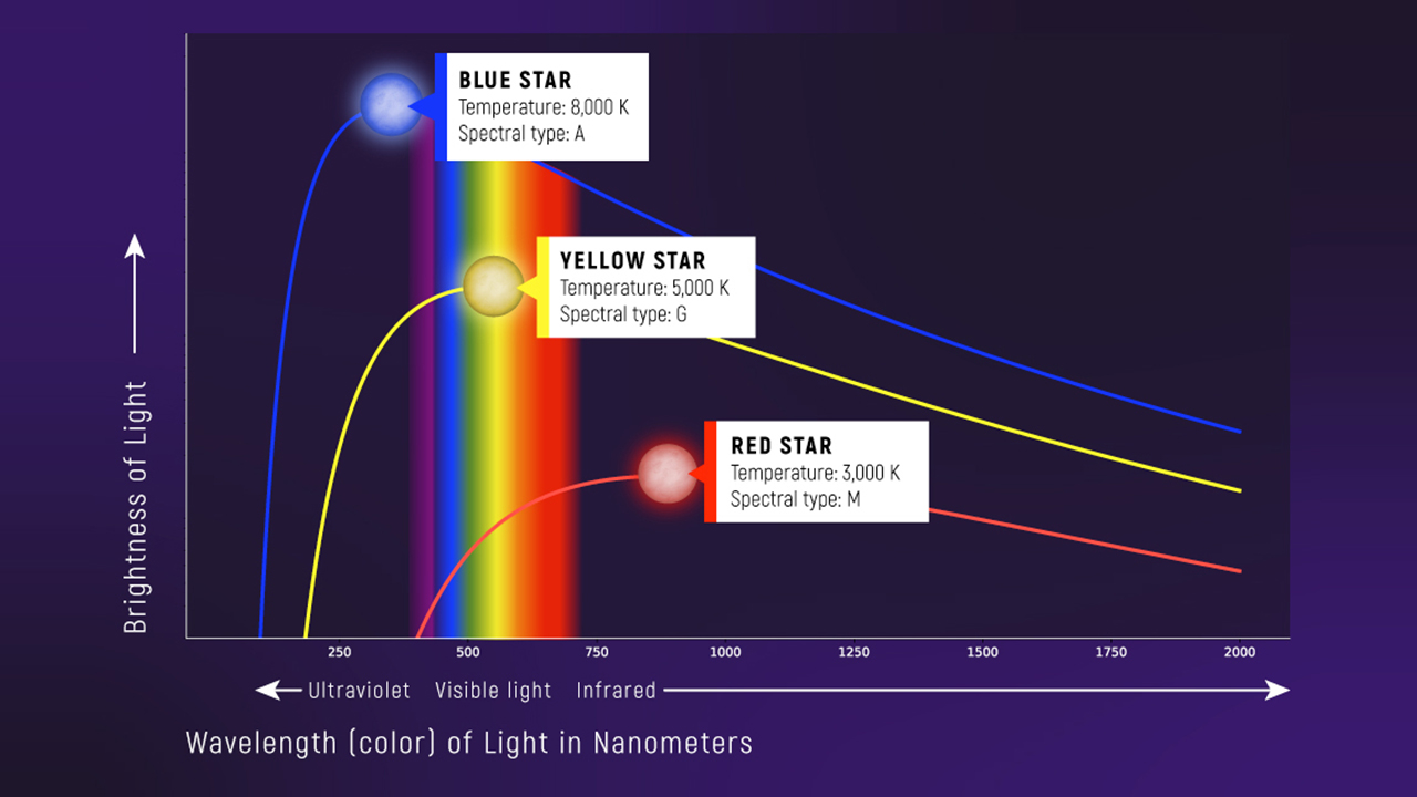
What to notice:

• Hotter curves peak at shorter wavelengths
• Hotter curves have much larger total area (more luminosity)

This is the demo, frozen.

UV Catastrophe: What Classical Physics Predicted

At long wavelength, classical physics gives the Rayleigh–Jeans form:

\[ B_\lambda \propto \frac{T}{\lambda^4} \]

If you extend that to \(\lambda \rightarrow 0\):

Warning

\(B_\lambda \rightarrow \infty\) → infinite energy output. That would mean hot objects radiate unlimited UV. The universe would be absurdly UV-bright.

Say ‘classical physics breaks’ — not ‘people measured wrong.’

Planck’s Move (1900): Quantization

Planck assumed energy exchange happens in packets:

\[ E = h\nu = hc\lambda^{-1} \tag{1}\]

Meaning:

• short wavelength ↔︎ high frequency ↔︎ high photon energy
• high-frequency photons are expensive
• so UV emission is suppressed

Important

That “UV cutoff” behavior you saw in the demo is quantum mechanics in action.

This is the historical ‘physics had to change’ moment.

The Fix: A Finite, Physical Spectrum

\[ B_\lambda(T)=\frac{2hc^2}{\lambda^5}\cdot\frac{1}{e^{hc/(\lambda k_B T)}-1} \tag{2}\]

Key behavior:

• Long wavelengths: classical approximation emerges
• Short wavelengths: exponential suppression prevents divergence
• Total emitted power becomes finite → stars can exist

No derivation today; HW3 has the limits.

Wien’s Law: Color → Temperature (the fast tool)

Wien’s displacement law (peak in \(B_\lambda\)):

\[ \lambda_{\text{peak}} = b T^{-1} \tag{3}\]

Interpretation:

• hotter → smaller \(\lambda_{\rm peak}\) (bluer peak)
• cooler → larger \(\lambda_{\rm peak}\) (redder peak)

Tip

Use ratio form whenever possible — constants cancel.

Wien Ratio Form (Exam-Safe)

From \(\lambda_{\rm peak} = b/T\):

\[ \frac{T_1}{T_2} = \frac{\lambda_{\rm peak,2}}{\lambda_{\rm peak,1}} \]

So relative to the Sun:

\[ \frac{T_\star}{T_\odot} = \frac{\lambda_{\rm peak,\odot}}{\lambda_{\rm peak,\star}} \]

This is the version I want you using under time pressure.

Ratio Example: 500 nm vs 250 nm

Given:

• \(\lambda_{\rm peak,\odot} \approx 500\,\text{nm}\)
• \(\lambda_{\rm peak,\star} \approx 250\,\text{nm}\)

Then:

\[ \frac{T_\star}{T_\odot} = \frac{500}{250} = 2 \Rightarrow T_\star \approx 2(5800\,\text{K}) \approx 1.16\times10^4\,\text{K} \]

Tip

Halving peak wavelength doubles temperature.

Make them say the direction out loud.

Quick Check: Direction

If \(\lambda_{\rm peak}\) shifts to a longer wavelength, the star is:

• hotter
• cooler
• unchanged in temperature
• impossible to classify

This prevents the classic sign flip.

Radius Inference: Solve Stefan–Boltzmann for \(R\)

From \[ L = 4\pi R^2 \sigma T^4 \]

Solve: \[ R = \left(\frac{L}{4\pi\sigma T^4}\right)^{1/2} \]

Warning

Common mistake: forgetting the \(1/2\) power (writing \(R^2\) by accident).

If they only remember one pitfall, it’s this.

Solar-Unit Form (Cleaner, Fewer Mistakes)

Divide by the Sun’s Stefan–Boltzmann law:

\[ \frac{L}{L_\odot} = \left(\frac{R}{R_\odot}\right)^2 \left(\frac{T}{T_\odot}\right)^4 \]

Solve for radius:

\[ \frac{R}{R_\odot} = \left( \frac{L/L_\odot}{(T/T_\odot)^4} \right)^{1/2} \]

Tip

This is the “no constants, no unit pain” form.

The Astronomer’s Decoder Ring (Today)

Observable \(\rightarrow\) Model \(\rightarrow\) Inference

1. Measure brightness + distance: \(F + d \rightarrow L\)
   
2. Measure color/peak: \(\lambda_{\rm peak} \rightarrow T\)
   
3. Combine: \((L, T) \rightarrow R\) via Stefan–Boltzmann

Credit: Course illustration (A. Rosen)

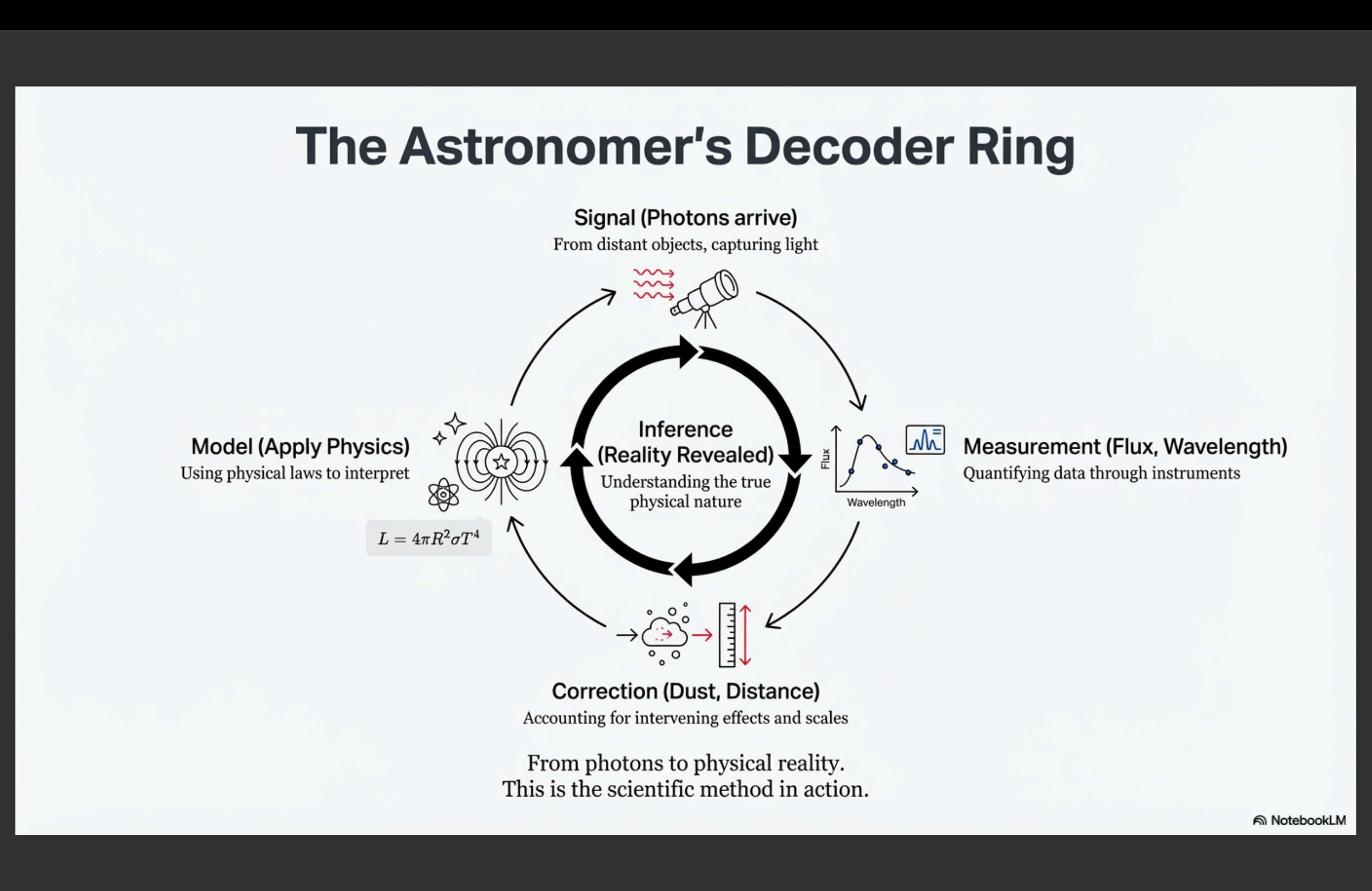
This is the thesis slide. Slow down here.

How Do We Know This Isn’t Just Math Magic?

We can validate radii with independent methods:

• Eclipsing binaries: geometry + timing gives radii directly
• Interferometry: angular size + distance → physical radius
• Spectral energy distributions: fit full spectrum for \(T\) and bolometric flux

Important

In astronomy, inference becomes knowledge when independent methods agree.

This is your scientific-method / epistemology anchor.

Betelgeuse: Qualitative Inference (words first)

Betelgeuse is:

• cooler than the Sun (\(T \sim 3500\,\text{K}\))
• incredibly luminous (\(L \sim 10^5 L_\odot\))

Cool surface means low \(F_\star=\sigma T^4\), yet total luminosity is huge.

Important

Only one way to reconcile both: enormous emitting area → large radius.

Force the logic chain in English before numbers.

Betelgeuse Scale (let this land)

Credit: ESO/L. Calçada

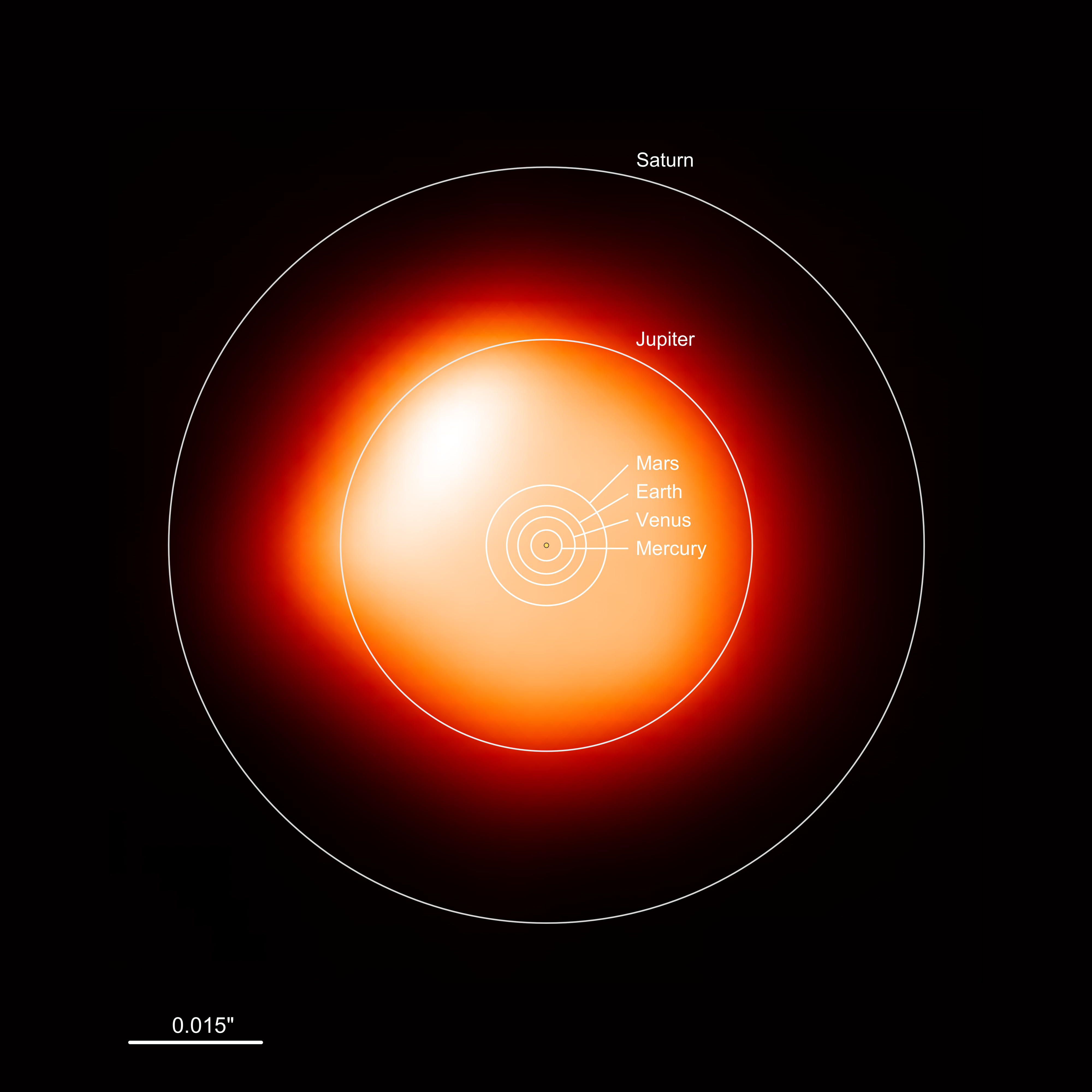
Order-of-magnitude radius:

\[ R \sim 10^3 R_\odot \]

Roughly hundreds to about a thousand solar radii.

Warning

Spoiler alert: Betelgeuse is an evolved massive star, a red supergiant.

Pause. Let them react. This is the emotional payoff.

Mini-Activity (8 minutes): Hotter, Same Luminosity

Work in pairs. Write one equation + one sentence.

A star has:

• \(L = L_\odot\)

• \(T = 2T_\odot\)

Start from:

\[ L \propto R^2 T^4 \]

Tasks:

1. Find \(R/R_\odot\).

2. Predict: bluer or redder than the Sun.

3. Place it relative to the Sun on the HR diagram (left/right, up/down).

Credit: ESO

Use this map for directional placement only.

Start timer. Cold-call for #1 and #3.

Mini-Activity Debrief

At fixed luminosity:

\[ R \propto T^{-2} \Rightarrow \frac{R}{R_\odot} = \left(\frac{T}{T_\odot}\right)^{-2} = (2)^{-2} = \frac{1}{4} \]

So the star is hotter (bluer) and smaller but with same \(L\).

Reinforce: same luminosity ≠ same size.

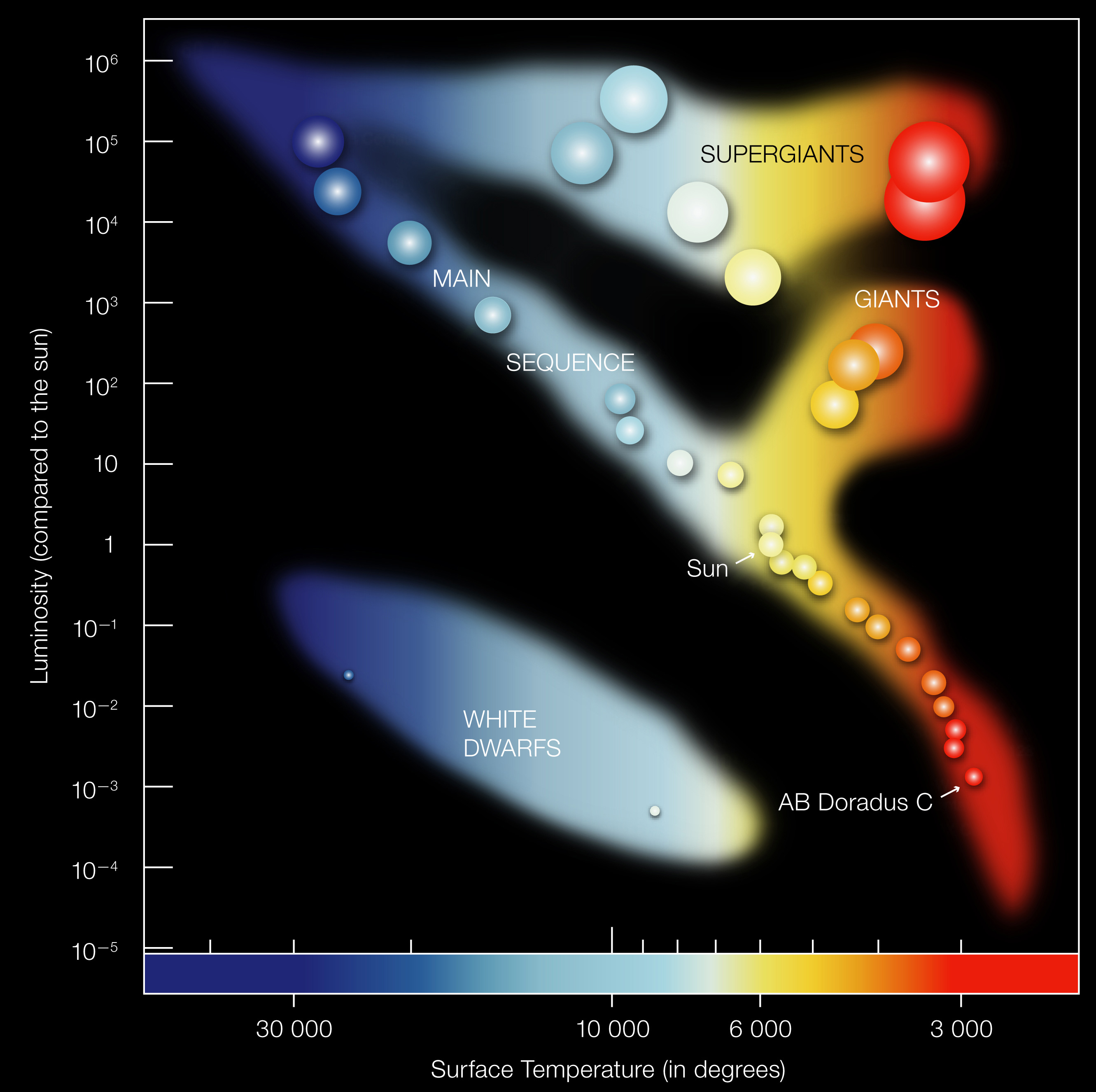
HR Diagram Preview: Radius Map in Disguise

Credit: ESO

Interpretation using \[ L \propto R^2T^4 \]

• Cool + luminous \(\rightarrow\) large \(R\) (giants/supergiants)
• Hot + dim \(\rightarrow\) small \(R\) (white dwarfs)

Hotter is to the left (historical convention).

Say the line: ‘HR diagram is a radius map in disguise.’

Synthesis Quiz: What Determines Apparent Brightness?

To decide whether Betelgeuse placed at \(10\,\mathrm{pc}\) would appear brighter or dimmer than Sirius, which quantities must you compare directly?

• surface flux and temperature
• luminosity and distance
• radius and peak wavelength
• color index and surface flux

Apparent brightness comparisons need \(L\) and \(d\).

Exit Ticket (2 sentences)

Write two sentences (this is your study summary):

1. “Color tells us ______ because ______.”
2. “At fixed luminosity, hotter means ______ radius because ______.”

Collect or have them self-check.

Summary Takeaways: The Intrinsic Triad

The three intrinsic stellar properties are:

• Luminosity \(L\): total power output
• Effective temperature \(T_{\text{eff}}\): surface temperature
• Radius \(R\): physical size

These form a closed physical relationship: \[ L = 4\pi R^2 \sigma T^4 \]

If you know any two, physics constrains the third.

Important

Astronomy is an inference machine: \[ \text{observables} \rightarrow \text{model} \rightarrow \text{physical reality} \]

\[ T \rightarrow 2T \quad \Rightarrow \quad L \rightarrow 16L \] \[ R \rightarrow 2R \quad \Rightarrow \quad L \rightarrow 4L \]

Reinforce that \(T^4\) is the dominant lever: temperature changes drive luminosity much more steeply than radius changes.

Summary Takeaways: Flux vs Surface Flux

Received flux (observer-dependent): \[ F = \frac{L}{4\pi d^2} \] Depends on distance \(d\).

This tells us how bright a star looks from Earth.

Surface flux (intrinsic): \[ F_\star = \frac{L}{4\pi R^2} = \sigma T^4 \] Depends on stellar properties, not observer location.

This tells us how intensely each cm\(^2\) of stellar surface radiates.

Warning

Key distinction: \(F\) changes when you move; \(F_\star\) changes only if the star changes.

Say explicitly: received flux is a geometric dilution effect, while surface flux is local stellar physics.

Summary Takeaways: The Inference Chain

\[ F + d \rightarrow L,\quad \lambda_{\rm peak} \rightarrow T,\quad (L,T) \rightarrow R \]

Use Wien’s law for temperature: \[ \lambda_{\rm peak} \propto \frac{1}{T} \]

Then solve Stefan-Boltzmann for radius: \[ R=\left(\frac{L}{4\pi \sigma T^4}\right)^{1/2} \]

Case-study conclusion (Rigel vs Betelgeuse):

• Similar luminosity can coexist with very different radii.
• Cooler stars must have much larger surface area to match high \(L\).
• This logic is what maps stars onto the H-R diagram as a radius structure.

Close by restating the thesis: stars are not points of light, they are constrained physical objects with inferable sizes.

Next Time

Next: spectral lines and classification refine temperature and reveal composition.

Today you built the core chain: \(F + d \rightarrow L\), \(\lambda_{\rm peak} \rightarrow T\), \((L,T)\rightarrow R\).

End with continuity + confidence.

Appendix (Optional, Study Support)

The next slides:

• Show why the Wien ratio form works algebraically
• Derive Wien’s law from the Planck function (optimization)
• Are not required for in-class problem solving
• Are fully fair game for conceptual exam questions

Warning

Optional appendix: requires comfort with derivatives and basic optimization.

This is here so students can study the logic, not because they need to memorize a full derivation.

Appendix A: Why the Wien Ratio Form Cancels the Constant

Start from Wien’s law:

\[ \lambda_{\rm peak} = \frac{b}{T} \]

Write it for two stars:

\[ \lambda_1 = \frac{b}{T_1}, \quad \lambda_2 = \frac{b}{T_2} \]

Take the ratio:

\[ \frac{\lambda_1}{\lambda_2} = \frac{(b/T_1)}{(b/T_2)} = \frac{T_2}{T_1} \]

Rearrange:

\[ \frac{T_1}{T_2} = \frac{\lambda_2}{\lambda_1} \]

Important

The constant \(b\) cancels automatically. That is why the ratio method is fast and safe.

If they forget the numerical constant, they can still solve ratio questions correctly.

Why Calculus Matters: Deriving Wien’s Law

Warning

Optional extension for interested students: this section uses calculus and is not required for this course.

Planck’s function (per wavelength form):

\[ B_\lambda(T) = \frac{2hc^2}{\lambda^5} \frac{1}{e^{hc/(\lambda kT)} - 1} \]

Goal: find the wavelength at the maximum, \(\lambda_{\rm peak}\).

\[ \frac{dB_\lambda}{d\lambda} = 0 \]

Credit: JWST/STScI

Peak-finding on this curve is exactly where calculus enters.

Start by pointing at the visual peak and say: “this is what the derivative is locating.”

Step 1: Define a Dimensionless Variable

Let:

\[ x = \frac{hc}{\lambda kT} \]

Then:

\[ \lambda = \frac{hc}{xkT} \]

We rewrite Planck’s function in terms of \(x\).

Step 2: Express the Peak Condition in Terms of \(x\)

After rewriting and differentiating (details skipped here for space), the peak condition becomes:

\[ 5(1 - e^{-x}) = x \]

This is a transcendental equation.

It cannot be solved analytically.

Step 3: Solve the Peak Equation (Numerically)

Peak condition:

\[ 5(1 - e^{-x}) = x \]

Numerical solution:

\[ x \approx 4.965 \]

This single number pins down where the Planck curve peaks.

Important

This is the calculus payoff: one equation, one number, one measurable prediction.

Point at the curve peak and connect it to the solved value of \(x\).

Step 4: Turn \(x\) into Wien’s Constant

Use the definition

\[ x = \frac{hc}{\lambda_{\rm peak} kT} \]

to get

\[ \lambda_{\rm peak} T = \frac{hc}{kx} \]

Substitute \(x \approx 4.965\):

\[ \lambda_{\rm peak} T = 2.898 \times 10^{-3}\ \mathrm{m\,K} = 2.898 \times 10^6\ \mathrm{nm\,K} \]

That constant is Wien’s displacement constant.

Tip

Why calculus matters: it generates the constant you use in real stellar temperature inference.

What This Derivation Really Means

• The peak of the Planck curve is determined by a balance between two effects.

• The \(\lambda^{-5}\) factor rises sharply at short wavelength.

• The exponential suppression term kills short-wavelength emission.

• The maximum occurs where those two competing effects balance.

• The number \(4.965\) encodes that balance.

Important

Wien’s law is not empirical magic. It falls directly out of quantum thermal physics.

This connects blackbody shape to quantization at a deeper level.

Long-Wavelength Limit (Rayleigh–Jeans)

When \(x = hc/(\lambda kT) \ll 1\):

\[ e^x \approx 1 + x \]

Planck reduces to:

\[ B_\lambda \propto \frac{T}{\lambda^4} \]

This matches classical physics.

Short-Wavelength Limit (Exponential Suppression)

When \(x \gg 1\):

\[ e^x - 1 \approx e^x \]

Planck becomes:

\[ B_\lambda \propto \lambda^{-5} e^{-hc/(\lambda kT)} \]

The exponential term suppresses UV emission.

Warning

This suppression is what prevents the ultraviolet catastrophe.

Why This Matters for Stellar Inference

Without Planck’s exponential cutoff:

• Total luminosity would diverge.
• Stefan-Boltzmann would not converge.
• Wien’s law would not exist.

Quantum mechanics makes stellar astrophysics possible.

Close the loop: QM \(\rightarrow\) finite spectrum \(\rightarrow\) usable temperature \(\rightarrow\) usable radius.