Spectra & Composition
What’s It Made Of, and How Is It Moving?
Learning Objectives
- Explain Kirchhoff’s three laws and predict which spectrum a source produces
- Interpret the Bohr model to explain why spectral lines have specific wavelengths
- Classify stars by spectral type (OBAFGKM) as a temperature sequence
- Apply the Doppler shift to measure stellar radial velocities
- Connect spectral absorption to the greenhouse effect
Read aloud. ~1 min. Students should note these — they map to what’s testable.
All stars are \({\sim}73\%\) hydrogen and \({\sim}25\%\) helium.
So why do their spectra look so different?
0–1 min. Let this sit for 5 seconds. Don’t answer yet.
This is the throughline question for the whole lecture. The answer (temperature controls which energy levels are populated) won’t land until Part 3, but planting it now gives students a reason to pay attention.
Today’s Roadmap
- Kirchhoff’s Laws — why stars show absorption spectra
- Spectral Lines — atomic fingerprints from the Bohr model
- OBAFGKM — a temperature sequence, not composition
- Doppler Shift — reading stellar motion from light
- Putting It Together — three clues from one spectrum
- Climate Connection — same physics, different scale
30 seconds. Quick orientation. Point to each item.
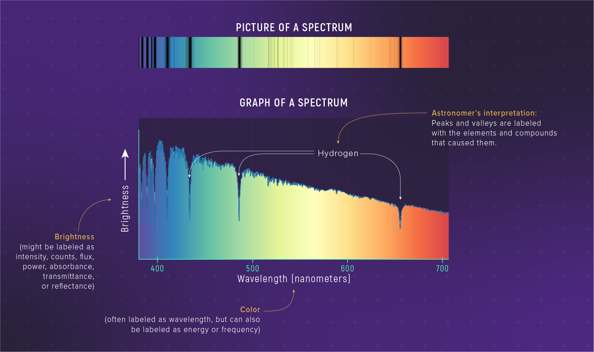
Kirchhoff’s Laws
Three spectra, three physical setups
Three Types of Spectra
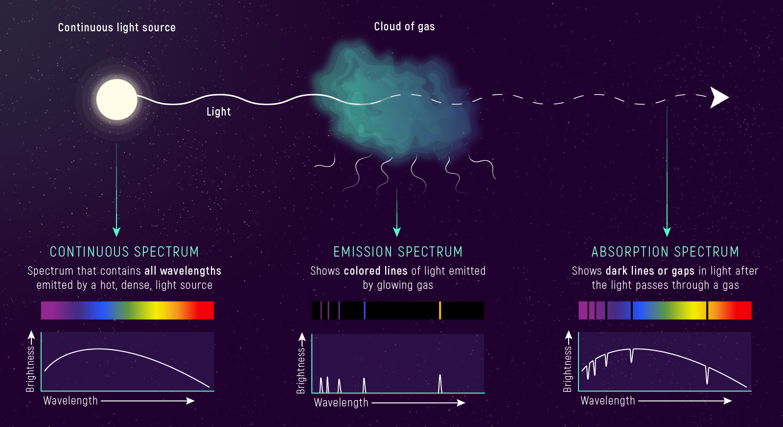
- Continuous — hot, dense source → all wavelengths (Planck curve)
- Emission — hot, low-density gas → bright lines on dark background
- Absorption — cooler gas in front of hot continuum → dark lines
The same gas produces emission OR absorption depending on what’s behind it.
2–3 min. Point to each type in the figure. Reveal the list, then the fragment. Emphasize that the physical setup — not the gas itself — determines which type you see.
Quick Label (30 seconds)
For each spectrum type, write down: (1) the type and (2) the physical setup in six words or fewer.
Example format:
- Continuous — hot, dense source emits all wavelengths.
- Emission — hot, thin gas emits bright lines.
- Absorption — cool gas blocks specific colors.
~3 min. 30-second micro-task. Let students write, then reveal the example answers. This cements the three types before formalizing them as Kirchhoff’s laws.
Kirchhoff’s Three Laws
- Hot, dense source → continuous spectrum (all wavelengths)
- Hot, low-density gas → emission lines (bright lines, dark background)
- Cooler gas in front of hot continuum → absorption lines (dark lines in rainbow)
The same gas absorbs at the same wavelengths it would emit.
3–4 min. Reveal one at a time. Stress law 3: the absorption wavelengths match the emission wavelengths — Kirchhoff noticed this empirically.
The Reverse Problem
In practice, you work Kirchhoff’s laws backwards:
Given a spectrum → infer the physical configuration.
- Dark lines in a rainbow? → cooler gas in front of a hotter continuum
- Bright lines on dark background? → hot, tenuous gas, no continuum behind it
- Smooth rainbow, no lines? → hot, dense source
This is the skill you’ll use for the rest of the course.
~4 min. Quick reframe. The “reverse problem” is the working-astronomer mindset: you start with data, not theory. You see a spectrum and deduce the physics. Stress that this is the same logic for every spectrum they’ll encounter.
Why Stars Show Absorption Spectra

Two-layer model:
- Photosphere (\(\tau \approx 1\)) — hot, dense → continuous spectrum (Law 1)
- Atmosphere (cooler, above) → absorbs at specific wavelengths (Law 3)
We see: a continuous rainbow with dark lines carved into it.
Temperature decreases outward — that’s why absorption, not emission.
4–5 min. Walk through the two-layer model. The photosphere is where optical depth \(\tau \approx 1\) — the depth where the star becomes opaque. The cooler atmosphere above it absorbs at specific wavelengths.
Two Myths to Kill Now
Myth 1: “Spectral type tells me what a star is made of.”
It doesn’t — not directly. Spectral type primarily reflects temperature. Stars of wildly different types have nearly identical compositions. (Part 3 will prove this.)
Myth 2: “A redshifted star looks red.”
It doesn’t. “Redshift” means lines shift to longer wavelengths — a fractional change of \({\sim}0.01\%\). A blue O star receding from you is still blue. (Part 4 makes this quantitative.)
~5 min. Deliver these as firm corrections. Students who build the wrong mental model here will struggle for weeks. These same myths appear in the reading’s “Two Myths to Kill Now” box — reinforce here so students hear it twice.
Observable → Model → Inference
- Observable: Dark lines at specific wavelengths in a stellar spectrum
- Model: Kirchhoff’s third law — cooler atmosphere absorbs from hotter photosphere
- Inference: The star has a hot interior surrounded by a cooler atmosphere
The dark lines are the key to everything that follows.
🔍 Spectrum Detective — Clue 0: The shape of the spectrum (continuous vs. lines, absorption vs. emission) tells you the physical setup of the source.
6–7 min. This is the O→M→I frame for the whole lecture. Every dark line encodes physics. The “Spectrum Detective” motif runs through the reading — plant the first clue here.
Prediction: Which Spectrum?
You look at a glowing neon sign through a spectrograph.
Commit to one answer:
Continuous spectrum — smooth rainbow
Emission spectrum — bright lines on dark background
Absorption spectrum — dark lines in a rainbow
7–8 min. Give 30 seconds. Cold-call 2 students.
Answer: (b) Emission. Neon is a hot, low-density gas (Kirchhoff’s law 2). No hot dense source behind it → no continuum to absorb from.
Spectral Lines as Atomic Fingerprints
The Bohr model and discrete energy levels
The Bohr Model: Discrete Energy Levels
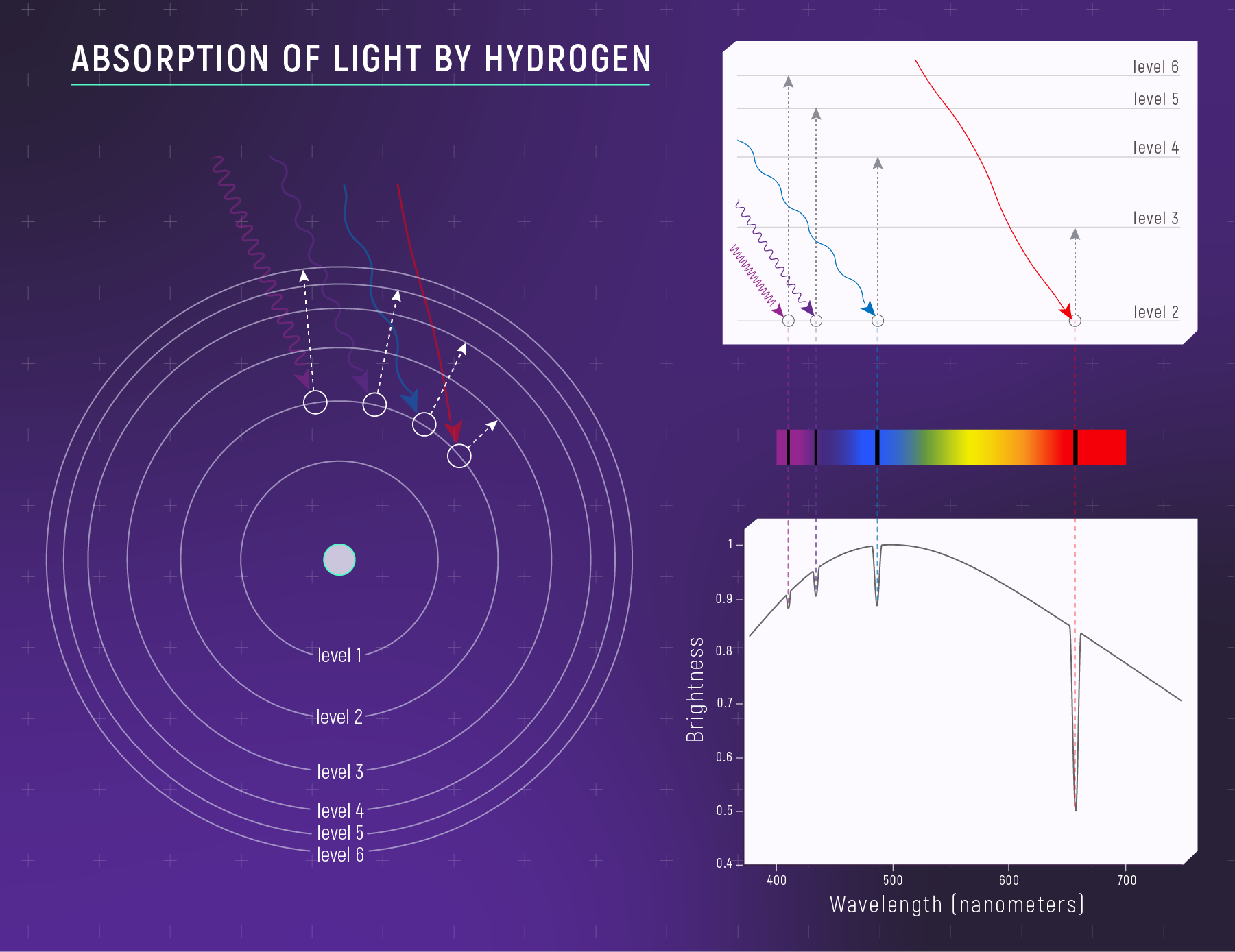
Electrons occupy specific energy rungs — they cannot hover between them.
10–12 min. Point to the energy levels in the diagram.
Key idea: electrons can only be at certain energies. To absorb a photon, the photon’s energy must exactly match a gap between levels. This is why absorption happens at specific wavelengths.
The Reverse: Emission
Same energy gaps → same wavelengths — whether absorbing or emitting.
~12 min. Quick. Same gaps, same wavelengths. This is why Kirchhoff’s observation works: the gas absorbs at the same wavelengths it emits.
Hydrogen Energy Levels
\[E_n = -\frac{13.6\ \text{eV}}{n^2}\]
- \(n = 1\) (ground state): \(E_1 = -13.6\ \text{eV}\) — most tightly bound
- \(n = 2\): \(E_2 = -3.4\ \text{eV}\)
- \(n \to \infty\): \(E = 0\) — electron is free (ionized)
Negative sign = the electron is bound. You must add energy to free it.
12–13 min. Walk through the levels slowly. The minus sign confuses students — address it directly. “More negative = more tightly bound.”
Spectral Lines Come from Transitions
When an electron jumps between levels:
\[\Delta E = |E_{\text{upper}} - E_{\text{lower}}|\]
. . .
The photon’s wavelength is set by the energy gap:
\[\lambda = \frac{hc}{\Delta E}\]
Different elements → different energy levels → different spectral lines.
13–14 min. This is the core mechanism. Each element has a unique set of energy levels, so each element produces a unique barcode of spectral lines.
The Balmer Series: Hydrogen’s Visible Fingerprint
Transitions to/from \(n = 2\):
| Transition | Name | Wavelength | Color |
|---|---|---|---|
| \(n = 3 \to 2\) | H\(\alpha\) | \(656\ \text{nm}\) | Deep red |
| \(n = 4 \to 2\) | H\(\beta\) | \(486\ \text{nm}\) | Blue-green |
| \(n = 5 \to 2\) | H\(\gamma\) | \(434\ \text{nm}\) | Violet |
| \(n = 6 \to 2\) | H\(\delta\) | \(410\ \text{nm}\) | Near-UV |
Energy gaps of \(\sim 1.9\text{–}3.0\ \text{eV}\) → visible wavelengths.
14–15 min. These are the most important spectral lines in stellar astronomy. H\(\alpha\) is the red glow in nebula photos.
Worked Example: Calculating H\(\alpha\)
Problem: Predict the wavelength of \(n = 3 \to 2\) in hydrogen.
. . .
Step 1 — Energy levels: \[E_3 = \frac{-13.6\ \text{eV}}{9} = -1.51\ \text{eV} \qquad E_2 = \frac{-13.6\ \text{eV}}{4} = -3.40\ \text{eV}\]
. . .
Step 2 — Energy gap: \[\Delta E = |-1.51\ \text{eV} - (-3.40\ \text{eV})| = 1.89\ \text{eV}\]
. . .
Step 3 — CGS conversion: (\(1\ \text{eV} = 1.602 \times 10^{-12}\ \text{erg}\)) \[\lambda = \frac{hc}{\Delta E} = \frac{1.986 \times 10^{-16}\ \text{erg·cm}}{3.03 \times 10^{-12}\ \text{erg}} = 6.56 \times 10^{-5}\ \text{cm} = 656\ \text{nm}\ \checkmark\]
15–16 min. Walk through step by step. Every intermediate value carries its unit — eV on every numerator, eV on every subtraction. This is the full CGS grind; the shortcut comes next.
The \(hc\) Shortcut — Your Default Tool
For any transition with energy gap \(\Delta E\) (in eV):
\[\lambda\ (\text{nm}) \approx \frac{1240\ \text{eV·nm}}{\Delta E\ (\text{eV})}\]
For H\(\alpha\):
\[\lambda \approx \frac{1240\ \text{eV·nm}}{1.89\ \text{eV}} \approx 656\ \text{nm}\ \checkmark\]
Same answer, one line. Use \(hc \approx 1240\ \text{eV·nm}\) freely unless a problem asks for CGS.
~17 min. This shortcut is designated as the default tool for ASTR 201. Students should memorize \(hc \approx 1240\ \text{eV·nm}\). The full CGS derivation is for “show your work” problems; this is for quick estimates and sanity checks.
Every Element Has a Unique Barcode
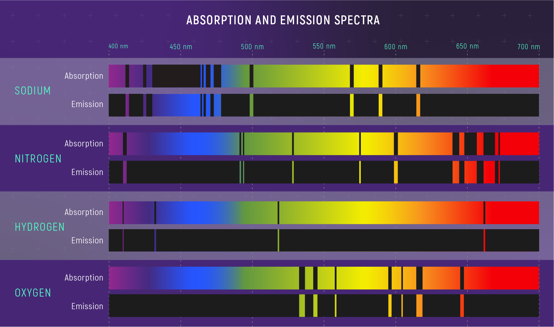
Match observed lines to laboratory wavelengths → identify the element.
🔍 Spectrum Detective — Clue 1: The positions of absorption lines tell you which elements are present — each element’s fingerprint is unique.
17–18 min. This is the payoff: we identify elements in stars by matching their spectral barcode to lab data. No need to visit the star.
Real Data: Altair’s Spectrum
Two tools in one observation: the curve gives temperature (Wien), the lines give composition.
18–19 min. Point to the smooth blackbody-like envelope → gives the temperature. Point to the dark dips → those are absorption lines, primarily hydrogen Balmer series. This is what a real stellar spectrum looks like when you spread starlight through a spectrograph. Altair is an A7V star — strong Balmer lines, as expected.
Quick Check: Spectral Lines
An absorption line appears at \(486.1\ \text{nm}\) in a star’s spectrum. Which element and transition is this?
- Helium, ground-state transition
- Hydrogen, \(n = 4 \to 2\) (H\(\beta\))
- Sodium, D-line transition
- Iron, ionized state
~22 min. Give 20–30 seconds.
Correct: \(486.1\ \text{nm}\) is H\(\beta\), the second Balmer line. Students should be learning to recognize these numbers.
OBAFGKM
A temperature sequence — not composition
The Harvard Computers
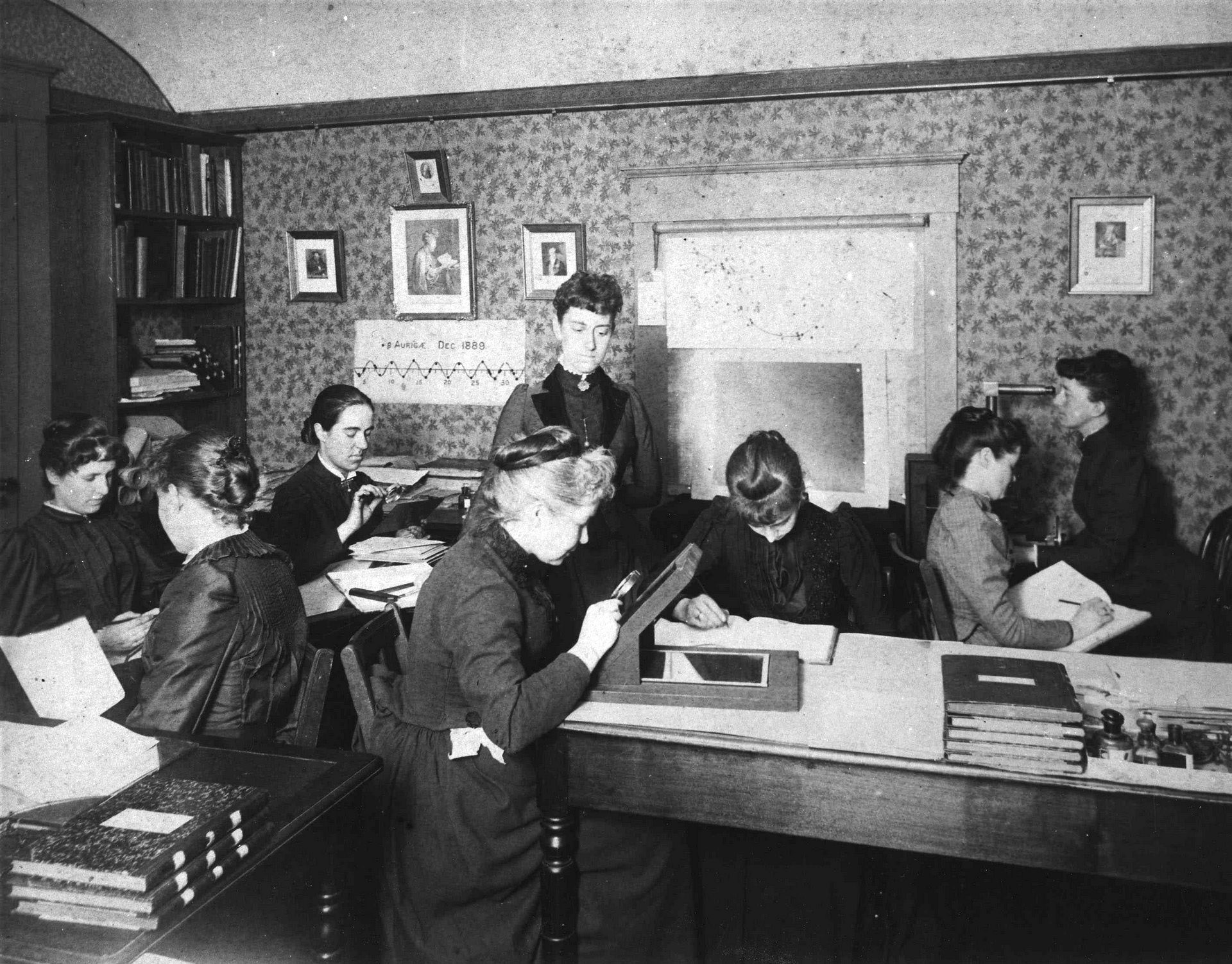
500,000 glass plates. Millions of spectra. No automation.
- Williamina Fleming — first classification system, 310 variable stars, Horsehead Nebula
- Annie Jump Cannon — 350,000 spectra classified, OBAFGKM sequence
- Antonia Maury — noticed line widths vary → luminosity class
Hired as cheap labor (25–50¢/hr, less than secretaries), denied telescope access — and they transformed astronomy.
22–23 min. Frame this as the “industrial data problem”: two technologies (spectroscopy + photography) created a data bottleneck. Pickering hired women because they were educated, available, and cheap. The classification work was NOT clerical — it required recognizing subtle patterns in noisy photographic data, statistical pattern recognition before formal statistics.
Data First, Theory Later
The Harvard classifications demanded explanation:
- 1925: Cecilia Payne-Gaposchkin proved stars are overwhelmingly hydrogen & helium — arguably the most important PhD in astronomy. Her advisor Russell called it “clearly impossible” before later admitting she was right.
- 1920s: Eddington’s stellar models explained OBAFGKM as a temperature sequence.
- 1938: Bethe’s nuclear fusion theory completed the picture.
The pattern was observed first. The physics was built to explain it.
This is Observable → Model → Inference in its purest historical form.
~24 min. This slide connects the Harvard Computers to the course’s O→M→I framework. The spectral sequence was empirical — the Boltzmann distribution and Saha equation came later to explain why it exists. This is how science usually works, even when textbooks present it the other way around.
The Spectral Sequence
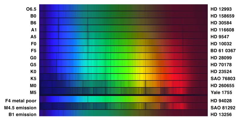
From top to bottom: O → B → A → F → G → K → M
- Hot (O): ionized helium lines
- Middle (A): strongest hydrogen Balmer lines
- Cool (M): molecular bands (TiO)
Spectral features change dramatically — but composition is nearly the same across all types.
Oh Be A Fine Guy/Girl, Kiss Me.
24–25 min. Walk through the sequence from O (hot, blue) to M (cool, red). Point to how the spectral features change dramatically even though composition is ~the same.
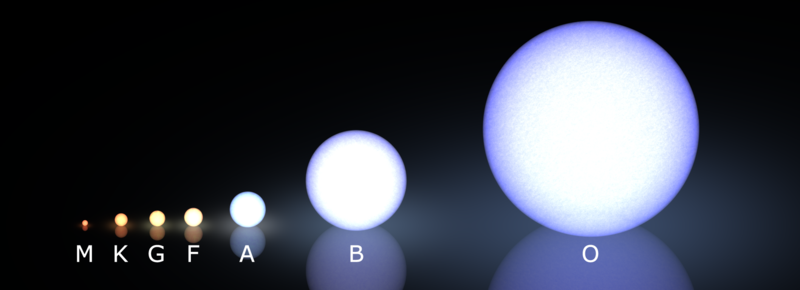
OBAFGKM at a Glance
| Type | Color | Temperature | Main-Seq. Prevalence | Dominant Features |
|---|---|---|---|---|
| O | Blue-violet | \(\gtrsim 30{,}000\ \text{K}\) | \(0.00003\%\) | Ionized helium |
| B | Blue-white | \(10{,}000\text{–}30{,}000\ \text{K}\) | \(0.13\%\) | Neutral helium, strong H |
| A | White | \(7{,}500\text{–}10{,}000\ \text{K}\) | \(0.6\%\) | Strongest H Balmer |
| F | Yellow-white | \(6{,}000\text{–}7{,}500\ \text{K}\) | \(3\%\) | Moderate H, weak metals |
| G | Yellow | \(5{,}200\text{–}6{,}000\ \text{K}\) | \(7.6\%\) | Weak H, strong metals |
| K | Orange | \(3{,}700\text{–}5{,}200\ \text{K}\) | \(12.1\%\) | Very weak H, molecular bands |
| M | Red-orange | \(\lesssim 3{,}700\ \text{K}\) | \(76.5\%\) | TiO molecular bands |
M dwarfs are \(76.5\%\) of all stars — too faint to see by eye.
25–26 min. Don’t read the whole table. Highlight three things:
- A stars have strongest H lines
- G stars (like the Sun) show strong metal lines
- M dwarfs dominate the galaxy by number
Four Knobs, One Spectrum
| What You Measure | What It Tells You |
|---|---|
| Line positions (which wavelengths are dark) | Composition — which elements are present |
| Line strength pattern (which species dominate) | Temperature → spectral type (OBAFGKM) |
| Line widths (narrow vs. broad) | Surface gravity / rotation → luminosity class |
| Metal line forest (amplitude relative to H) | Metallicity (heavy-element abundance) |
Temperature is the dominant knob — it controls line strengths so powerfully that it can mask composition differences entirely.
~26 min. This table is from the reading. Temperature is the first-order effect; metallicity and gravity are second-order. The table gives students a mental checklist for reading any spectrum.
Why Temperature Controls Line Strength
- For H absorption: electron must already be in \(n = 2\)
- Fraction in \(n = 2\) depends on temperature: \(\propto e^{-\chi_2/k_BT}\)
- Too cool (M stars): almost no atoms in \(n = 2\) → weak H lines
- Just right (A stars): maximum population in \(n = 2\) → strongest H lines
- Too hot (O stars): hydrogen is ionized → no neutral H → weak H lines
26–28 min. This is the hardest conceptual point. Walk slowly.
The Boltzmann factor \(e^{-\chi/kT}\) with \(\chi_2 = 10.2\ \text{eV}\) means you need \(T \sim 10{,}000\ \text{K}\) to populate \(n = 2\) significantly. But go too hot and hydrogen ionizes entirely. The “sweet spot” is A-star temperatures.
Predict First: Which Type Wins?
All stars are \({\sim}73\%\) hydrogen. Hydrogen Balmer absorption requires electrons already in \(n = 2\), which is \(10.2\ \text{eV}\) above the ground state.
At which spectral type — O, A, G, or M — would you expect the strongest Balmer lines, and why?
Commit to an answer before I show you.
~28 min. Give 30 seconds. Do NOT reveal the answer — let the next slide do that. This is a “Predict First” moment from the reading. Students who commit to a prediction learn more from the explanation.
The Goldilocks Problem: A Balmer Line Peak
Two competing effects at work:
- Excitation (\(\propto e^{-\chi_2/k_BT}\)): hotter → more atoms in \(n = 2\)
- Ionization: hotter → more atoms lose electrons entirely
. . .
| Temperature | Excitation | Ionization | Balmer strength |
|---|---|---|---|
| \(3{,}000\ \text{K}\) (M) | Very low | Negligible | Weak — no \(n=2\) |
| \(10{,}000\ \text{K}\) (A) | High | Moderate | Peak — sweet spot |
| \(35{,}000\ \text{K}\) (O) | Very high | Nearly complete | Weak — no neutral H |
Balmer strength rises, peaks at A stars, then falls — a competition, not monotonic growth.
28–30 min. Draw this out as a sketch if chalkboard is handy: x-axis = temperature, y-axis = Balmer line strength. The curve rises from M, peaks at A, and falls again at O. This non-monotonic behavior is what makes the spectral sequence surprising and what Cecilia Payne-Gaposchkin had to explain.
Prediction: Why Weak H Lines?
An M star (\(T \approx 3{,}000\ \text{K}\)) has weak hydrogen Balmer lines.
Which explanation is correct?
M stars have very little hydrogen
M stars are too cool — almost no H atoms in the \(n = 2\) state
M stars are so hot that hydrogen is ionized
M stars are too far away to show lines
~31 min. Give 30 seconds. Cold-call.
Answer: (b). All stars have \({\sim}73\%\) hydrogen. But at \(3{,}000\ \text{K}\), the Boltzmann factor puts almost no atoms in \(n = 2\), so Balmer absorption is extremely weak.
This directly answers the hook question from the beginning!
The Spectral Sequence Is Temperature
- Do O stars have more helium? No — same composition. Temperature ionizes H and excites He.
- Do A stars have more hydrogen? No — same abundance. Temperature puts H into \(n = 2\).
- Do M stars lack hydrogen? No. Temperature keeps H atoms in \(n = 1\) (ground state).
Same atoms. Different temperatures. Different spectra.
🔍 Spectrum Detective — Clue 2: The pattern of line strengths tells you temperature (spectral type). Strong Balmer? \({\sim}10{,}000\ \text{K}\). TiO bands? Below \({\sim}3{,}700\ \text{K}\).
31–32 min. This is the punchline that answers the opening question. Land it clearly. Clue 2 completes the temperature inference.
Quick Check: Spectral Type
Two stars have identical composition. Star X is spectral type A; Star Y is spectral type M. What’s different?
- Star X has more hydrogen
- Star Y has more metals
- Star X is hotter, so more H atoms occupy the \(n = 2\) level
- Star Y is closer, so lines appear weaker
~33 min. Give 20 seconds.
Correct: temperature controls level populations, not composition.
Metallicity: A Secondary Effect
Metallicity (\(Z\)) = mass fraction of elements heavier than helium.
- Sun: \(Z_\odot \approx 0.014\) — about \(1.4\%\) “metals”
- High-\(Z\) stars: more and stronger metal absorption lines
- Low-\(Z\) stars: “cleaner” spectra with fewer metal lines
But metallicity is second-order for classification. Two stars at the same temperature with different \(Z\) have the same spectral type — the metal line strengths differ, but which species dominates is set by temperature.
33–34 min. Quick slide. Metallicity matters for detailed chemical abundance work, but it doesn’t change the spectral type itself. The OBAFGKM system is primarily a temperature sequence.
Fun fact: in astronomy, everything heavier than helium is a “metal.” Carbon, oxygen, iron — all “metals.”
Beyond Temperature: What Line Widths Reveal
- Giants/supergiants: low-density atmospheres → narrow spectral lines
- Dwarfs (main-sequence): compact, dense atmospheres → broad spectral lines
G2V (Sun) and G2Ib (supergiant): same temperature, wildly different size and luminosity.
34–35 min. Introduce the Morgan–Keenan luminosity class briefly. The Roman numeral (V = dwarf, III = giant, I = supergiant) encodes surface gravity, which spectroscopists read from line widths. An M supergiant (Betelgeuse, M2Ia) can be more luminous than a hot O dwarf — temperature ≠ luminosity.
We’ll use this extensively when we build the full H–R diagram in Lectures 5–6.
The Doppler Shift
Reading stellar motion from light
Doppler: Wavelength Shifts from Motion
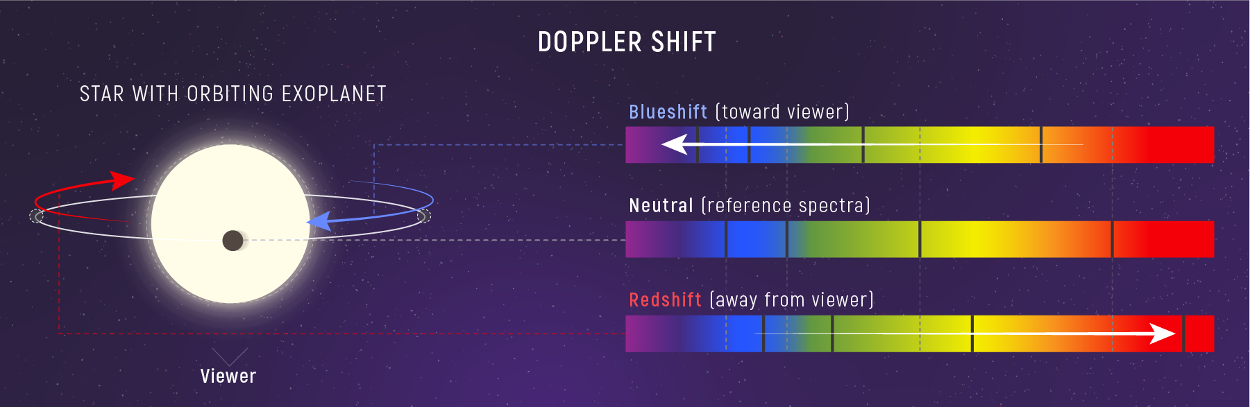
Motion along the line of sight shifts all spectral lines:
- Receding → lines shift to longer wavelengths (redshift)
- Approaching → lines shift to shorter wavelengths (blueshift)
Typical stellar velocities: \(10\text{–}100\ \text{km/s}\) → shifts of only \({\sim}0.01\text{–}0.03\%\), but measurable.
36–37 min. Connect to sound analogy (ambulance siren) but keep it brief — go straight to the formula on the next slide.
The Doppler Formula
\[\frac{\Delta\lambda}{\lambda_0} = \frac{v_r}{c}\]
- \(\Delta\lambda = \lambda_{\text{obs}} - \lambda_0\) — the shift
- \(v_r\) — radial velocity (+ = receding, − = approaching)
- \(c = 3.0 \times 10^5\ \text{km/s}\) — speed of light
Redshift (\(\Delta\lambda > 0\)): source receding | Blueshift (\(\Delta\lambda < 0\)): source approaching
Diagnostic: A real Doppler shift moves all lines by the same fraction \(\Delta\lambda/\lambda_0\). If only one line shifts — it’s a misidentification, not motion.
37–38 min. Both sides are dimensionless ratios. Stress: typical stellar velocities are \(10\text{–}100\ \text{km/s}\), so shifts are tiny (\({\sim}0.01\text{–}0.03\%\)) but measurable. The diagnostic about all lines shifting by the same fraction is a crucial practical check — students will need this when analyzing real spectra.
Worked Example: Radial Velocity from H\(\alpha\)
Problem: H\(\alpha\) observed at \(656.5\ \text{nm}\) (rest: \(656.3\ \text{nm}\)). Approaching or receding?
. . .
Step 1 — Direction: \(\lambda_{\text{obs}} > \lambda_0\) → redshifted → receding
. . .
Step 2 — Shift: \(\Delta\lambda = 656.5\ \text{nm} - 656.3\ \text{nm} = 0.2\ \text{nm}\)
. . .
Step 3 — Velocity: \[v_r = c \times \frac{\Delta\lambda}{\lambda_0} = (3.0 \times 10^5\ \text{km/s}) \times \frac{0.2\ \text{nm}}{656.3\ \text{nm}} \approx 91\ \text{km/s}\]
A \(0.03\%\) shift → \({\sim}91\ \text{km/s}\). Tiny shift, huge velocity.
38–39 min. Walk each step. Unit check: (km/s) × (nm/nm) = km/s ✓. Emphasize how a \(0.2\ \text{nm}\) shift is barely perceptible but translates to \({\sim}91\ \text{km/s}\) because \(c\) is enormous.
Quick Check: Doppler Direction
H\(\beta\) (rest: \(486.1\ \text{nm}\)) is observed at \(485.9\ \text{nm}\). The star is…
- Approaching (blueshifted — observed wavelength is shorter)
- Receding (redshifted)
- Stationary (no shift)
- Rotating (broadened)
~39 min. Give 20 seconds.
\(\lambda_{\text{obs}} < \lambda_0\) → blueshift → approaching. The velocity would be \(v_r = c \times (-0.2\ \text{nm}/486.1\ \text{nm}) \approx -123\ \text{km/s}\).
The Doppler Wobble in Action
~39 min. Play the video (~1 min). It shows a planet orbiting its host star and the resulting Doppler wobble — the star’s radial velocity oscillates as the planet tugs it back and forth. Watch how the spectrum shifts blueward and redward in sync with the orbit. This sets up the TPS on the next slide: students will now compute the wobble themselves.
Doppler Unlocks Masses
If a star is in a binary system, its radial velocity oscillates as it orbits.
Measure the oscillation period and amplitude → infer the companion’s mass.
Lecture 4: Binary orbits + Doppler → stellar masses.
🔍 Spectrum Detective — Clue 3: The shifts of line positions — every line offset by the same fraction — tell you the star’s radial velocity.
42–43 min. Forward pointer. Doppler isn’t just a velocity tool — it’s the most direct route to stellar masses, which determine everything about stellar evolution.
Putting It Together
Three clues from one spectrum
One Spectrum, Four Inferences
| Observable | What we measure | What we infer |
|---|---|---|
| Line positions (which wavelengths are dark) | Wavelengths matched to lab data | Composition |
| Line strength pattern (which species dominate) | Relative strengths | Temperature → spectral type |
| Line shifts (offset from lab wavelengths) | Doppler shift \(\Delta\lambda/\lambda_0\) | Radial velocity |
| Line widths (narrow vs. broad) | Pressure/rotational broadening | Surface gravity → luminosity class |
Composition, temperature, motion, and size — from a single observation.
🔍 Spectrum Detective — Case Closed. All clues collected: composition (Clue 1), temperature (Clue 2), velocity (Clue 3). Three independent measurements, one observation.
43–44 min. This is the synthesis moment. Four pieces of information from one spectrum. The Spectrum Detective motif from the reading wraps up here.
Multi-Clue Diagnosis
Observed: \(T \approx 9{,}500\ \text{K}\), strong Balmer lines, weak metals, H\(\alpha\) at \(656.1\ \text{nm}\)
. . .
(a) Spectral type: \({\sim}9{,}500\ \text{K}\) + strong Balmer → type A
. . .
(b) Velocity: \(\Delta\lambda = 656.1\ \text{nm} - 656.3\ \text{nm} = -0.2\ \text{nm}\) → blueshifted → approaching \[v_r = (3.0 \times 10^5\ \text{km/s}) \times \frac{-0.2\ \text{nm}}{656.3\ \text{nm}} \approx -91\ \text{km/s}\]
. . .
(c) What else do we need? Distance → luminosity → radius. Time-series Doppler → mass.
44–45 min. This worked example ties everything together. Reveal progressively. Each step uses a different tool from the lecture.
Try It Tonight: Read a Real Spectrum
Open the SDSS SkyServer Quick Look.
Enter: Plate 285, MJD 51930, Fiber 164 (a classic A star).
- Continuum shape — does it rise toward blue or red?
- Absorption lines — can you spot H\(\alpha\) (\(656\ \text{nm}\)) and H\(\beta\) (\(486\ \text{nm}\))?
- Line shifts — are lines at rest wavelengths, or offset?
You’ve just done real spectroscopy. Every line encodes the same physics from Parts 1–4.
~45 min. This is a “try it tonight” prompt from the reading’s 2-Minute Micro-Lab. If time permits and you have a projector, you can pull this up live. Otherwise, encourage students to explore on their own. The SDSS spectrum viewer is free and requires no login.
The Module 2 Inference Chain
| Lecture | New Tool | What It Unlocks |
|---|---|---|
| 1 | Parallax → distance | Distance, then luminosity |
| 2 | Color → temperature; Stefan-Boltzmann | Radius |
| 3 | Spectral lines | Composition, refined \(T\), velocity |
| 4 | Binary orbits + Doppler | Mass |
| 5–6 | Magnitudes + HR diagram | Full classification |
Five properties from photons alone. Mass needs one more tool.
46–47 min. Show where we are in the semester arc. After Lecture 4, we’ll have everything we need for the full H–R diagram.
Spectroscopy Meets Climate
Same physics, different scale
Planetary Energy Balance
At equilibrium: power absorbed from star = power radiated by planet.
\[T_{\text{eq}} = 279\ \text{K} \times (1-A)^{1/4} \times \left(\frac{d}{1\ \text{AU}}\right)^{-1/2}\]
For Earth (\(A = 0.3\), \(d = 1\ \text{AU}\)):
\[T_{\text{eq}} = 279\ \text{K} \times (0.70)^{1/4} \times 1 = 279\ \text{K} \times 0.915 = 255\ \text{K} = -18°\text{C}\]
Earth’s actual average: \(288\ \text{K} = +15°\text{C}\). Something warms us by \(33\ \text{K}\).
47–48 min. The ratio method makes this quick. Emphasize: \(255\ \text{K}\) is well below freezing — without the greenhouse effect, Earth would be an ice ball.
Predict First: What Warms Earth?
Earth’s equilibrium temperature is \(255\ \text{K}\) — well below freezing.
The observed average is \(288\ \text{K}\) — above freezing.
What must the atmosphere be doing to account for that \(33\ \text{K}\) difference?
Think about Kirchhoff’s third law applied to a planet instead of a star.
~47 min. Give 20–30 seconds. The atmosphere is the “cool gas” absorbing from the “hot continuum” (Earth’s surface thermal emission). Students should connect: the same law that explains stellar absorption lines also explains planetary warming. Don’t answer yet — the next slide does.
The Greenhouse Effect: Kirchhoff’s Law 3 for Planets
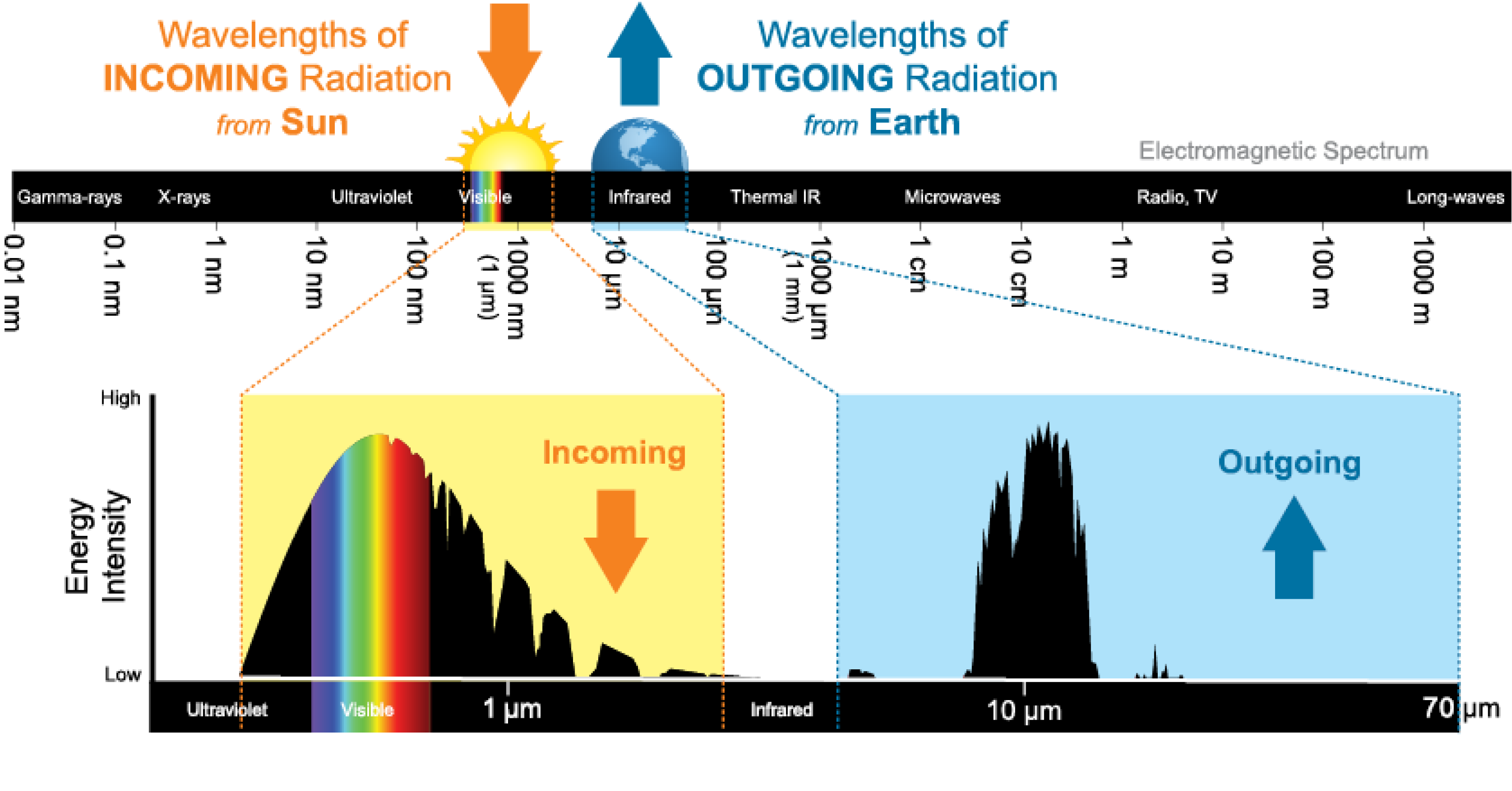
Two Planck curves:
- Sun → Earth peaks at ~0.5 μm (visible) — passes through atmosphere
- Earth → space peaks at ~10 μm (IR) — blocked by greenhouse gases
CO\(_2\), H\(_2\)O, CH\(_4\) absorb outgoing IR and re-emit some back down → surface warms.
This IS Kirchhoff’s Law 3: atmosphere = “cool gas” absorbing from the “hot continuum” (Earth’s surface).
48–49 min. Point to the two Planck curves in the figure. The atmosphere is transparent at visible wavelengths but opaque at thermal IR — that asymmetry is the entire greenhouse mechanism.
A Tale of Three Planets
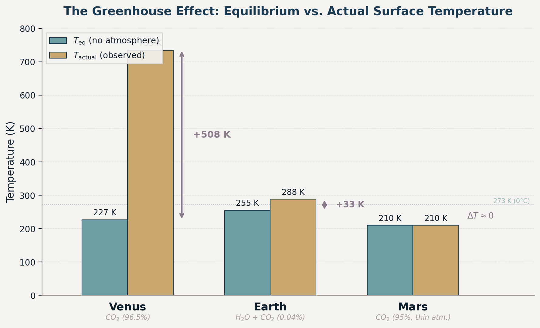
| Planet | \(T_{\text{eq}}\) (K) | Actual \(T\) (K) | Greenhouse warming |
|---|---|---|---|
| Venus | \(227\) | \(735\) | \(+508\ \text{K}\) |
| Earth | \(255\) | \(288\) | \(+33\ \text{K}\) |
| Mars | \(210\) | \(210\) | \({\sim}0\ \text{K}\) |
Same star, similar compositions. Atmosphere thickness makes all the difference.
49–50 min. Venus: runaway greenhouse, CO₂ at \(92\ \text{bar}\), hot enough to melt lead. Mars: CO₂ atmosphere but only \(0.6\%\) of Earth’s pressure → negligible greenhouse. Earth: just right — for now.
Note the paradox: Venus has a LOWER equilibrium temperature than Earth (high albedo reflects most sunlight), yet it’s \(460°\text{C}\) at the surface. That’s how powerful the greenhouse effect is.
CO\(_2\)’s 15 \(\mu\text{m}\) Band
CO\(_2\) absorbs at 15 \(\mu\text{m}\) — right where Earth’s thermal radiation peaks.
50–51 min. Point to the 15 μm absorption dip. This is the same quantum mechanics as hydrogen Balmer lines — molecular energy levels producing absorption at specific wavelengths. Adding more CO₂ deepens and broadens this band, trapping more outgoing IR.
CO₂ has gone from 280 ppm (pre-industrial) to ~425 ppm. The physics of why this matters has been understood since Tyndall (1861) and Arrhenius (1896).
Try It: Mars’s Equilibrium Temperature
Mars: \(d = 1.52\ \text{AU}\), \(A = 0.25\)
\[T_{\text{eq}} = 279\ \text{K} \times (1-0.25)^{1/4} \times \left(\frac{1.52\ \text{AU}}{1\ \text{AU}}\right)^{-1/2}\]
\((0.75)^{1/4} \approx 0.930 \qquad (1.52)^{-1/2} \approx 0.811\)
\[T_{\text{eq}} \approx 279\ \text{K} \times 0.930 \times 0.811 \approx 210\ \text{K}\]
Mars’s actual surface temperature is \({\sim}210\ \text{K}\). \(T_{\text{eq}} \approx T_{\text{surface}}\) — the greenhouse effect is negligible. Why? CO\(_2\) dominates (\(95\%\)), but the atmosphere is only \(0.6\%\) of Earth’s pressure. Too thin to trap significant IR.
51–52 min. Walk through the ratio method. Students should be comfortable with this from Lecture 2. The punchline: same greenhouse gas (CO₂) as Venus, but thin atmosphere → no warming. Atmospheric pressure matters as much as composition.
Quick Check: Greenhouse Physics
The greenhouse effect warms Earth because…
- CO\(_2\) absorbs incoming visible sunlight
- The ozone layer traps heat
- Atmospheric gases absorb outgoing infrared radiation and re-emit some downward
- Earth’s core heats the surface
~53 min. Give 20 seconds.
Correct: greenhouse gases absorb outgoing IR (not incoming visible), re-emit in all directions including downward. This is Kirchhoff’s law 3.
Two More Confusions to Clear Up
- “Stronger lines = more of that element.” Not necessarily. Line strength depends primarily on temperature — which levels are populated — not abundance. An A star doesn’t have more hydrogen than an M star; it just has the right \(T\) to populate \(n = 2\).
- “Absorption lines make a star dimmer.” Negligibly. Absorbed photons are re-emitted in random directions (resonant scattering). Total luminosity is conserved; the spectrum just has narrow dark features carved into it.
(Recall: we killed Myths 1 and 2 — spectral type ≠ composition, and redshift ≠ red star — at the start.)
54–55 min. Two confusions, not four — the other two were moved to “Two Myths to Kill Now” early in the lecture. Students have already internalized those; these two are the subtler traps.
What Spectra Can’t Tell Us (Directly)
- Mass — need binary orbits + Doppler (Lecture 4)
- Distance — need parallax or other distance indicator (Lecture 1)
- Age — need stellar evolution models (Module 3)
- Tangential velocity — Doppler gives only the radial component
Spectra are powerful — but not omnipotent. Every tool has limits.
55–56 min. Quick limitations slide. Keeps students honest about what one observation can and can’t do. Sets up why we need binary stars (Lecture 4) and the H–R diagram (Lectures 5–6).
Good question to pose: “If you only have a spectrum of an isolated star, can you determine its mass?” Answer: no — you get \(T_\text{eff}\) and composition, but mass requires either a binary orbit or a model-dependent mass–luminosity relation, which itself needs a distance measurement.
Summary: Key Takeaways
- Kirchhoff’s laws connect spectral appearance to physical conditions — stars show absorption spectra because of their temperature gradient
- Spectral lines are atomic fingerprints — energy levels set wavelengths
- OBAFGKM is a temperature sequence — same composition, different excitation
- Doppler shift converts wavelength shifts to velocities — \(\Delta\lambda/\lambda_0 = v_r/c\)
- Greenhouse effect is Kirchhoff’s law 3 applied to planets — same physics, different scale
56–57 min. Read through once. Each takeaway maps to a learning objective.
The Takeaway
If you forget everything else from today, remember this:
One spectrum → composition, temperature, velocity.
A star’s light is an autobiography — if you know how to read it.
~57 min. Let this land. This is the core message of the entire lecture.
Next Time: Binary Stars & Stellar Masses
Lecture 4: We put the Doppler shift to work on binary stars.
- Radial velocity oscillations → orbital period + amplitude
- Kepler’s laws → stellar masses
- Mass is the property that determines a star’s entire life story
The last fundamental property — and the most important one.
57–58 min. Build anticipation for Lecture 4. Mass determines luminosity, lifetime, fate — everything.
Questions?
Common questions at this point:
- “How do we know the lab wavelengths are right?” — Measured precisely since 1859
- “Can we determine composition from just one line?” — Need multiple lines for confidence
- “Do all stars have absorption spectra?” — Most, but emission-line stars exist (Be stars, Wolf-Rayet)
58–60 min. Leave remaining time for questions. Address the hook question one final time: “Same composition, different spectra — because temperature controls which energy levels are populated.”