Weighing Stars
Binary Orbits Reveal the Master Variable
Learning Objectives
- Explain why mass is the most fundamental stellar property and why it cannot be measured from a single star’s light alone
- Describe visual, spectroscopic, and eclipsing binary systems and what each reveals about the orbit
- Apply Newton’s version of Kepler’s third law to binary star orbits to determine the total system mass
- Use the center-of-mass condition and radial velocity amplitudes to determine individual stellar masses
- Interpret the mass-luminosity relation and explain why mass is the “master variable” for main-sequence stars
\[ L \propto M^{3.5} \]
~1 min. Read aloud. These map directly to the reading’s learning objectives and to the five summary takeaways at the end.
Mass controls everything about a star.
But you can’t weigh a star from its light.
0–1 min. Let this sit for 5 seconds. This is the paradox that drives the entire lecture. “Luminosity, temperature, radius, lifetime, how it dies — all set by mass. And mass is the one thing you can’t read from the photons.”
The Measurement Paradox
You can measure:
- Luminosity (distance + flux)
- Temperature (spectrum)
- Radius (Stefan–Boltzmann)
- Composition (spectral lines)
You cannot measure:
- Mass
Mass controls everything — but it is not uniquely encoded in the photons.
Today’s Roadmap
- The Hidden Variable — why mass matters most, and why it’s invisible
- Binary Stars — nature’s mass laboratories (visual, spectroscopic, eclipsing)
- Extracting Masses — Kepler III + center of mass = individual masses
- The Mass-Luminosity Relation — the most important empirical law in stellar astrophysics
- Module 2 Complete — the full inference chain from photons to stellar properties
~1–2 min. Quick orientation. Point to each item. “Today completes the Module 2 toolkit — after this, we can characterize every fundamental property of a star from its light.”
Mass Detective
The suspect controls everything — but mass is not uniquely encoded in the light.
~2–3 min. Introduce the running motif. “We’re opening a case today. The suspect is mass — it controls luminosity, temperature, radius, lifetime, and death. But it has no fingerprint in the light. No spectral line, no color, no brightness reveals it. We need a different kind of evidence.”
The Hidden Variable
Why mass is the most important property you can’t see
~3 min. Section divider. Transition to Part 1.
Two Stars, One Question
| Property | \(0.5\,M_\odot\) star | \(10\,M_\odot\) star | Ratio |
|---|---|---|---|
| Luminosity | \(\sim 0.09\,L_\odot\) | \(\sim 3 \times 10^3\,L_\odot\) | \(3 \times 10^4\!\times\) |
| Surface temperature | \(\sim 3{,}800\,\text{K}\) | \(\sim 2.5 \times 10^4\,\text{K}\) | \(\sim 7\times\) |
| Radius | \(\sim 0.5\,R_\odot\) | \(\sim 6\,R_\odot\) | \(\sim 12\times\) |
| Main-sequence lifetime | \(\sim 60\,\text{Gyr}\) | \(\sim 20\,\text{Myr}\) | \(\sim 3 \times 10^3\!\times\) |
| Death | White dwarf | Supernova | — |
A factor of 20 in mass changes luminosity by \(3 \times 10^4\!\times\) and determines life vs. death.
Mass is the master variable.
~4–5 min. Let the table sink in. “A factor of 20 in mass produces a factor of 30,000 in luminosity, reduces the lifetime by a factor of 3,000, and completely changes the endpoint. Mass determines everything.”
Predict: Two Bodies Orbiting
From Module 1, Lecture 3: Kepler’s third law for a planet orbiting a star contains the star’s mass:
\[P^2 = \frac{4\pi^2\, r^3}{G\, M}\]
What changes when both objects have comparable mass — like two stars orbiting each other?
- Nothing — the formula stays the same
- Replace \(M\) with \(M_1 + M_2\) and \(r\) with the total separation \(a\)
- The formula doesn’t apply to two stars
~7–8 min. Give 30 seconds. Cold-call. Answer: (b). This previews the binary Kepler III they’ll derive shortly. Students should remember the gist from Module 1.
The Only Way Out
Photons do not encode mass. Gravity does.
If we want mass, we must observe gravity in action.
Observable signature of gravity: Motion.
~8–9 min. Transition slide. “If photons don’t encode mass, then gravity has to do the work. Gravity leaves one observable trace: motion.”
Binary Stars
Nature’s mass laboratories
~9 min. Section divider. Transition to Part 2.
Most Stars Have Partners
- Roughly half of all Sun-like stars are in binary or multiple systems
- For massive O and B stars: 70–90% binary fraction
- Binary stars are the norm, not the exception
Without binaries, we could not measure stellar masses at all. The mass-luminosity relation — and much of our understanding of stellar physics — would be inaccessible.
~10 min. Quick facts. “Binaries are not rare curiosities — they’re the majority, especially for massive stars. And they’re the only direct way to measure stellar masses.”
Explore: Binary Orbits
Open the Binary Orbits explorer
~10–12 min. Open the link and give students 60 seconds to explore. Key observation to draw out: the heavier star barely moves; the lighter star swings wide. This primes the seesaw analogy and the center-of-mass condition they’ll see in Part 3.
Visual Binaries: Resolved on the Sky
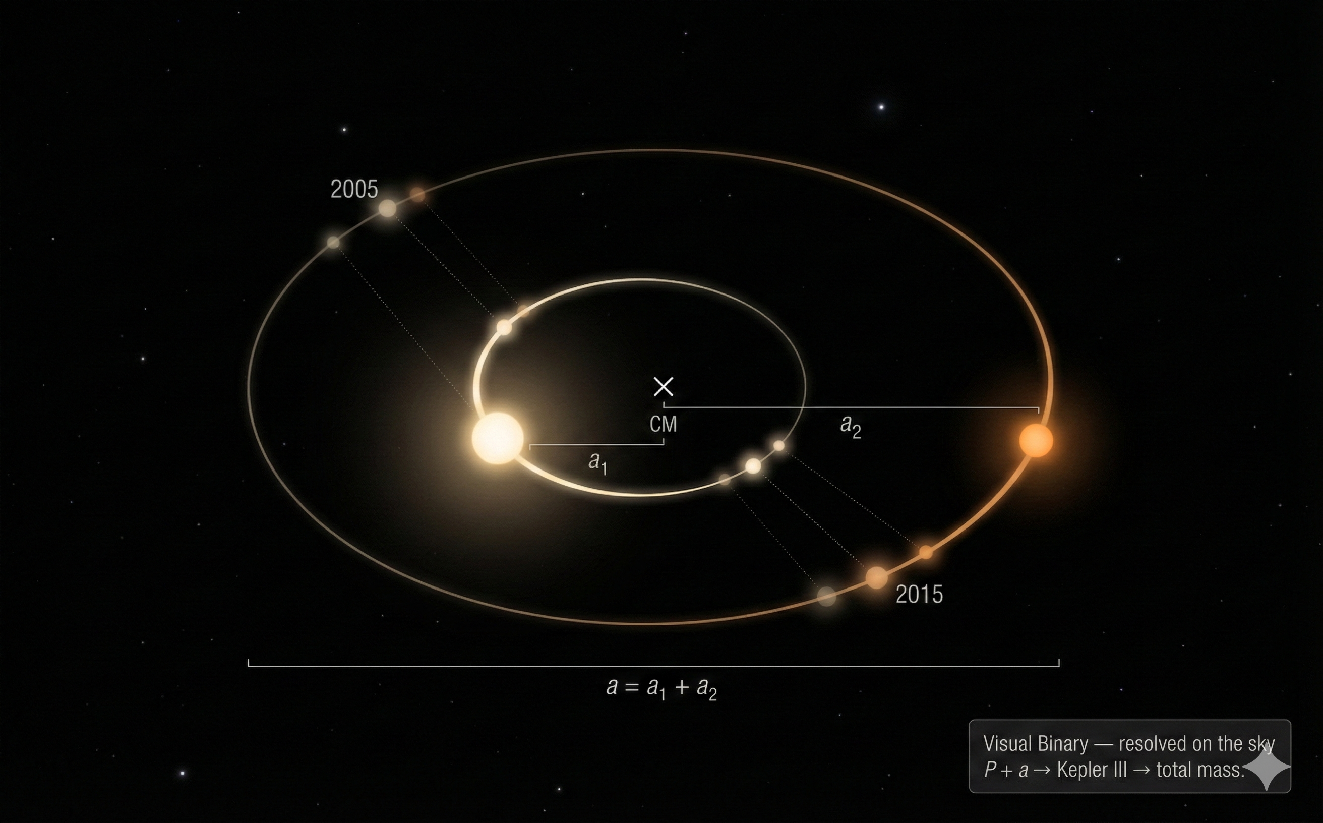
- Resolved as separate stars in a telescope
- Track positions over years/decades
- What they give us:
- Orbital period \(P\)
- Angular separation → physical separation \(a\) (with distance from parallax)
- Kepler III → total mass \(M_1 + M_2\)
Limitation: Requires wide separations (long periods — often decades) and nearby systems. Rare in practice.
~13–14 min. Point to the figure: heavier star traces smaller orbit, closer to center of mass. “This requires patience — orbital periods of decades or centuries. And you need the distance from Lecture 1’s parallax to convert angular orbits to physical separations.”
Sirius A + B: The Classic Visual Binary
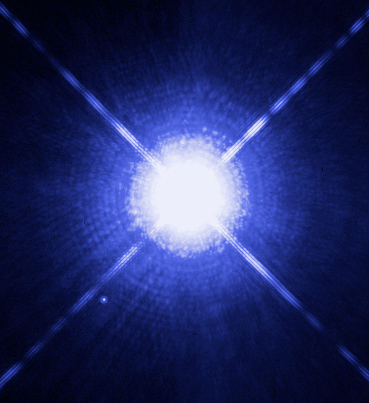
- Sirius A: \(2.06\,M_\odot\), A-type main sequence. Sirius B: \(1.02\,M_\odot\), white dwarf. \(P = 50.1~\text{yr}\), \(d = 2.64~\text{pc}\).
- In 1844, Bessel predicted an invisible companion from the wobble of Sirius A’s proper motion — 18 years before anyone saw it.
- Mass inferred from gravity before the companion was even observed.
- Mass Detective — Clue 1: Watch the sky. Visual binaries give \(P\) and \(a\) → total mass. But they’re rare and slow. We need more tools.
~14–15 min. “Bessel inferred mass from motion — exactly the strategy we’re learning. The companion turned out to be one of the most extraordinary objects in stellar astronomy: nearly the Sun’s mass crammed into a volume the size of Earth.”
Spectroscopic Binaries
Doppler Reveals the Orbit
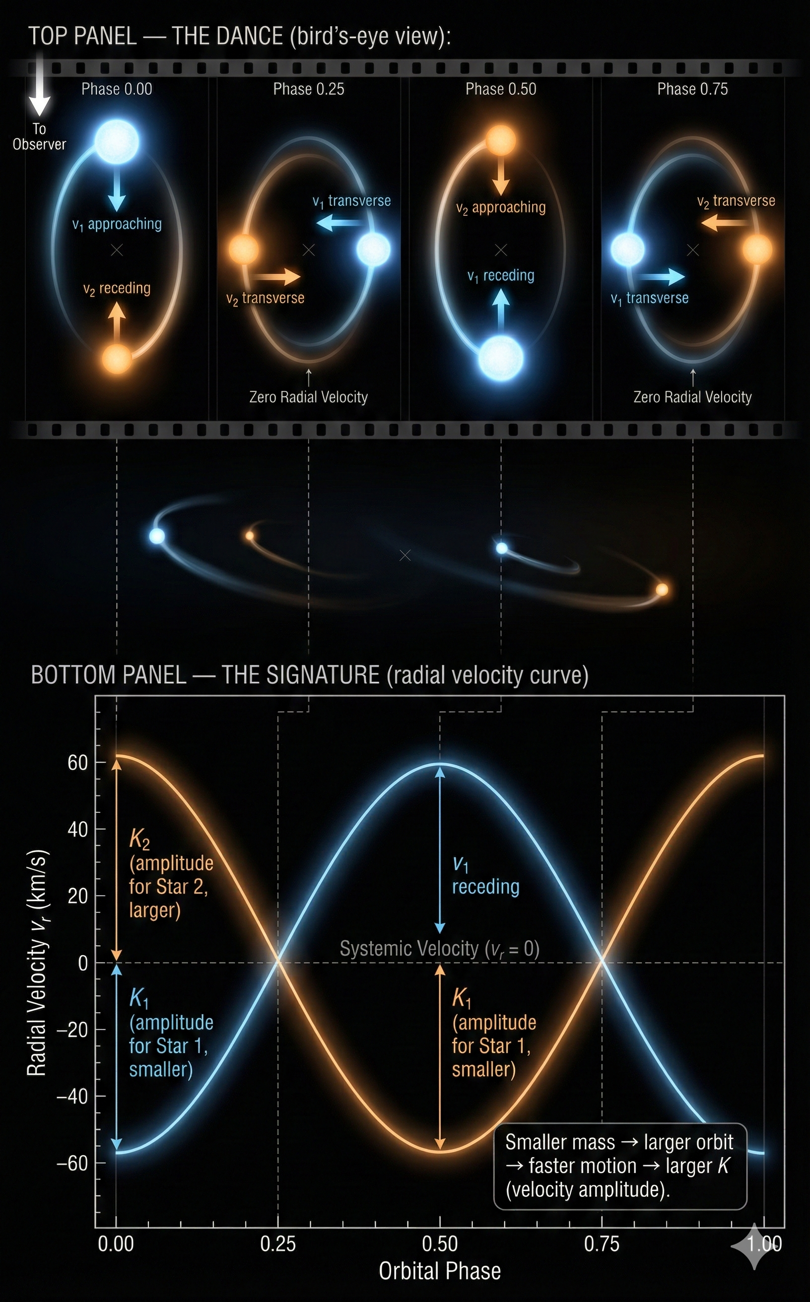
- Too close to resolve visually — but Doppler works
- Star orbits center of mass → spectral lines wobble
- Lecture 3 connection: Doppler shifts convert to radial velocity via
\[ \frac{\Delta \lambda}{\lambda_0} = \frac{v_r}{c} \]
now we track those velocities over time to trace the orbit - What they give us: - Orbital period \(P\) (from oscillation period) - Velocity amplitude \(K\) (from Doppler shift) - Works for close pairs at any distance
~16–17 min. Point to the RV curves in the figure. “This is the Doppler formula from Lecture 3 — now applied to trace orbits over time. The star with the larger \(K\) moves faster, which means it’s less massive — closer to the outer edge of the orbit.”
Connection: Exoplanet Radial Velocity
Same Doppler physics as RV exoplanets.
Key difference:
- Exoplanet case: \(M_{\text{planet}} \ll M_{\star}\)
- Binary case: \(M_1 \sim M_2\)
Both use:
\[ \frac{\Delta \lambda}{\lambda_0} = \frac{v_r}{c} \]
Binary stars are the symmetric version of exoplanet RV.
Single-Lined vs. Double-Lined
SB1 — Single-Lined
Only one star’s spectral lines are visible (companion too faint).
Get \(K_1\) only → mass constraint, not full mass ratio.
SB2 — Double-Lined
Both stars’ lines visible, shifting in opposite directions.
Get \(K_1\) AND \(K_2\) → mass ratio directly.
Mass Detective — Clue 2: Read the Doppler shifts. Periodic oscillations give \(P\) and \(K\) — but we only see the line-of-sight component. The orbital inclination is still hidden.
~17–18 min. “SB2 is the goal — two sets of lines moving in antiphase. When star 1 is blueshifted, star 2 is redshifted, and vice versa. That gives us both velocity amplitudes.”
Eclipsing Binaries
Light Curves Reveal Geometry
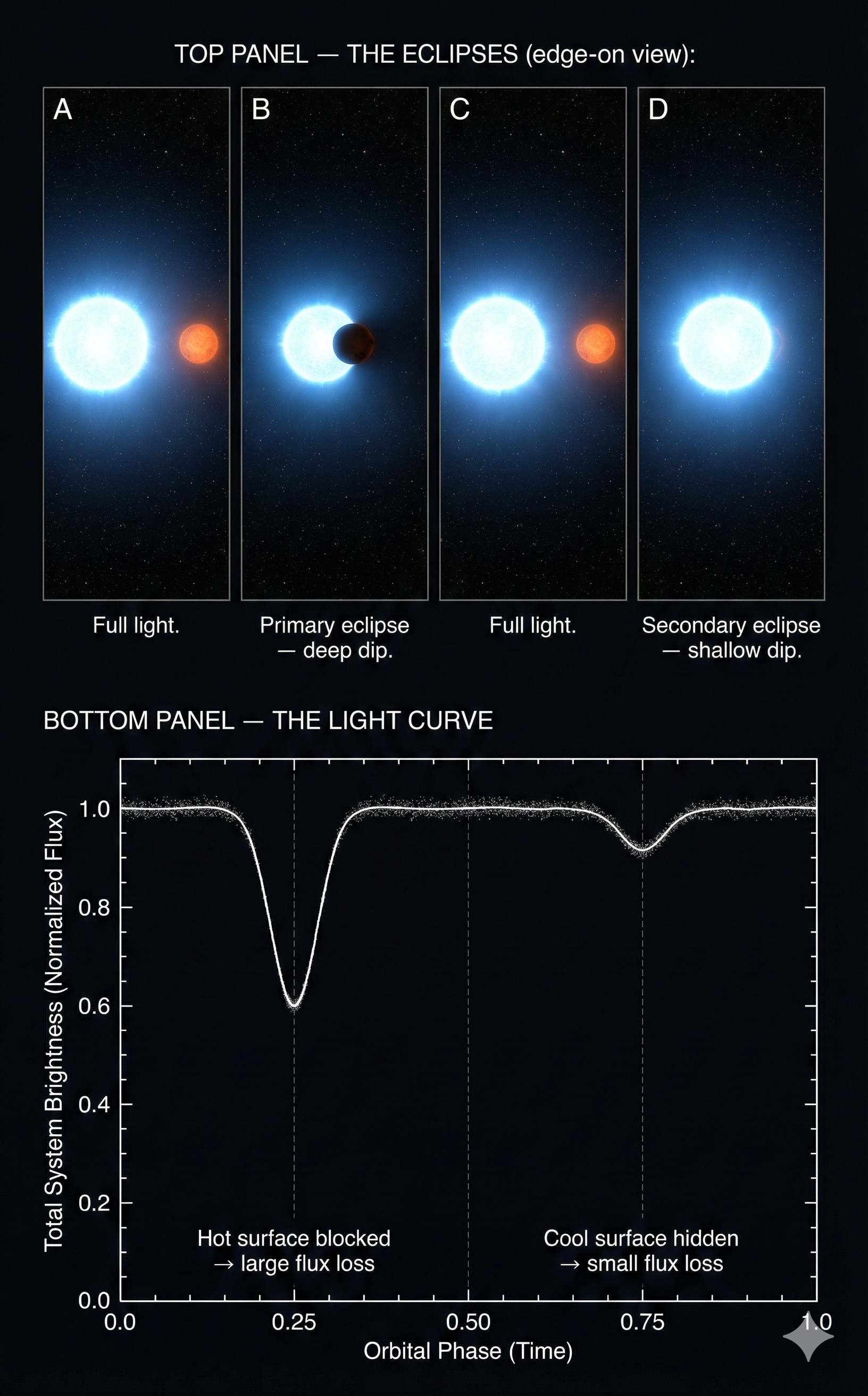
- Orbit nearly edge-on (\(i \approx 90°\)) → stars pass in front of each other
- Periodic brightness dips → light curve
- What they give us:
- Period \(P\)
- Inclination \(i \approx 90°\)
- Relative stellar radii
- Temperature ratio
The key unlock: eclipses tell us \(i \approx 90°\) — removing the biggest uncertainty.
~19–20 min. Point to the primary and secondary eclipses. Deep dip = hotter star blocked by cooler star. Shallow dip = cooler star hidden behind hotter star. “The inclination was the missing piece — eclipses fix it.”
The Gold Standard: Eclipsing + SB2
A system that is both an eclipsing binary and a double-lined spectroscopic binary gives us everything:
- Period \(P\), velocity amplitudes \(K_1\) and \(K_2\)
- Inclination \(i \approx 90°\)
- Both stellar radii \(R_1\), \(R_2\) and temperature ratio \(T_1/T_2\)
- Mass uncertainties of 1–2% — the most precise stellar mass measurements available
Mass Detective — Clue 3: Watch the light curve. Eclipses nail the inclination. Combine Clues 2 + 3 in the same system → we can measure everything. The blind spot is closed.
~20–21 min. Brief slide. “Eclipsing SB2 = the dream dataset. These are rare, but they’re the gold standard for stellar mass measurement.”
When This Method Fails
- Face-on orbit → no Doppler signal
- SB1 → mass ratio incomplete
- Non-eclipsing SB2 → absolute masses uncertain
- Post–main-sequence stars → mass–luminosity relation breaks
Every inference method has blind spots.
Ranking Challenge
Rank the following by how completely they determine stellar masses:
- Visual
- SB1
- SB2
- Eclipsing
- Eclipsing + SB2
1 = least information
5 = most complete mass determination
Be ready to name one missing parameter for your #1 and #5 choices.
~21–22 min. Give 45 seconds. Collect rankings before revealing or discussing. Keep the focus on what each method constrains vs. leaves ambiguous.
Binary Types at a Glance
| Binary Type | How Detected | What It Gives | What It Misses |
|---|---|---|---|
| Visual | Resolved orbit | \(P\), \(a\) (with distance), mass ratio (if both orbits measured) | Long baselines; nearby systems |
| Spectroscopic | Doppler curve | \(P\), \(K_1\) (and \(K_2\) for SB2) | Inclination \(i\) unknown |
| Eclipsing | Light-curve dips | \(P\), \(i \approx 90^\circ\), radius ratio, \(T\) ratio | Edge-on geometry required |
| Eclipsing + SB2 | Both datasets | \(M_1\), \(M_2\), \(R_1\), \(R_2\), \(T_1/T_2\) | Rare alignment + bright lines |
Each type adds a piece of the puzzle. The combination solves everything.
~22–23 min. Don’t read the whole table — highlight the progression. “Visual gives the sky orbit. Spectroscopy gives velocities. Eclipses give inclination. Put them together and every unknown is determined.”
Extracting Masses
From orbital measurements to stellar masses in four steps
~25 min. Section divider. Transition to Part 3. “We have the observational tools. Now: how do we go from measured quantities — \(P\), \(K_1\), \(K_2\) — to stellar masses?”
Predict: The Seesaw
In a spectroscopic binary, Star 1 has \(K_1 = 80~\text{km/s}\) and Star 2 has \(K_2 = 200~\text{km/s}\).
Which star is more massive?
Which star traces a larger orbit around the center of mass?
Hint: think about a seesaw — where does the heavy person sit?
~26 min. Give 30 seconds. Cold-call. Don’t reveal the answer yet — let the next slides derive it. The heavy person sits close to the pivot and barely moves (small orbit, small \(K\)). The light person sits far from the pivot and swings wide (large orbit, large \(K\)). So Star 1 is heavier.
Step 1: Kepler III for Binaries
In Module 1, you had:
\[ P^2 = \frac{4\pi^2 r^3}{G M} \]
for a planet orbiting a star.
For two stars with comparable masses, Newton’s full two-body form is:
\[ P^2 = \frac{4\pi^2\, a^3}{G(M_1 + M_2)} \tag{1}\]
\(a\) = total separation between the two stars
\(a = a_1 + a_2\)
- \(P\) = orbital period
- \(a = a_1 + a_2\) = total orbital separation
- \(M_1 + M_2\) = total system mass
What changed? \(M \to M_1 + M_2\) (both masses matter) and \(r \to a\) (total separation).
~27–28 min. Walk through slowly. “This is Module 1’s Kepler III, upgraded for two massive bodies. Both contribute to the gravitational interaction. The separation is between the two stars, not from either star to the center of mass.”
From Period and Separation to Total Mass
Rearranging Kepler III:
\[ M_1 + M_2 = \frac{4\pi^2\, a^3}{G\, P^2} \]
. . .
Measure \(P\) and \(a\) → get the total mass.
. . .
But we still need to split \(M_1\) from \(M_2\). That requires a second equation.
~28 min. Quick slide. Sets up the need for Step 2.
Step 2: The Center of Mass
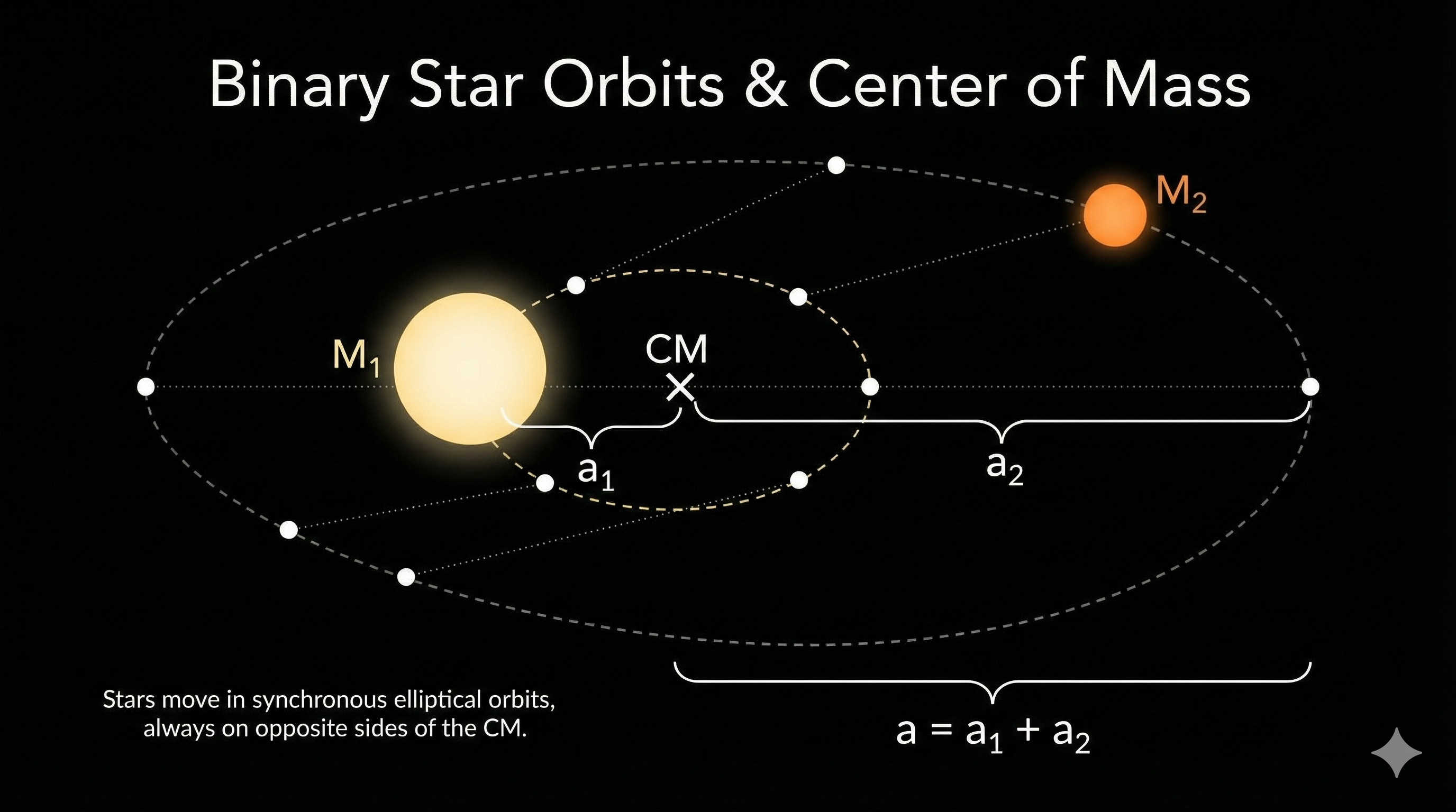
\[ M_1\, a_1 = M_2\, a_2 \tag{2}\]
The more massive star has the smaller orbit — it barely moves. The lighter star swings wide.
\[\frac{M_1}{M_2} = \frac{a_2}{a_1}\]
Mass ratio = inverse ratio of orbital radii.
~29–30 min. Point to the figure: the heavy star is near the center of mass, the light star is far away. “Like a seesaw — the heavy side is close to the pivot.” This answers the prediction from two slides ago.
Check Your Prediction
Back to the seesaw: \(K_1 = 80~\text{km/s}\), \(K_2 = 200~\text{km/s}\).
Star 2 moves faster → it’s farther from the center of mass → it’s the lighter star.
Star 1 moves slower → closer to the center of mass → it’s the heavier star.
Did your prediction match? The seesaw analogy works: heavy side barely moves, light side swings wide.
~28 min. Quick callback to the prediction. “If you got this right, you already understand the center-of-mass condition intuitively. Now let’s make it quantitative with velocities.”
Derive the Mass Ratio
Given:
\[ M_1 a_1 = M_2 a_2 \]
\[ v = \frac{2\pi a}{P} \]
Show that:
\[ \frac{M_1}{M_2} = \frac{v_2}{v_1} \]
Take 60 seconds. No calculators.
Step 3: Connecting Velocities to Orbits
For circular orbits:
\[ v_1 = \frac{2\pi a_1}{P}, \qquad v_2 = \frac{2\pi a_2}{P} \]
Same period:
\[ \frac{v_1}{v_2} = \frac{a_1}{a_2} = \frac{M_2}{M_1} \]
Doppler observables:
\[ K_1 = v_1 \sin i, \qquad K_2 = v_2 \sin i \]
\[ \frac{K_2}{K_1} = \frac{v_2 \sin i}{v_1 \sin i} = \frac{v_2}{v_1} \]
\(\sin i\) cancels.
\[ \frac{M_1}{M_2} = \frac{K_2}{K_1} \]
The mass ratio comes directly from RV amplitudes, independent of inclination.
~31–33 min. Three reveals. The key insight: \(\sin i\) cancels in the ratio. “Even without knowing the orbital inclination, we get the mass ratio from the Doppler measurements alone. That’s powerful.”
The Inclination Problem
Spectroscopy measures \(v \sin i\).
So inferred masses appear as \(M \sin^3 i\) (lower limits).
If the binary eclipses: \(i \approx 90^\circ \Rightarrow \sin i \approx 1\).
- Face-on (\(i = 0^\circ\)): no Doppler signal
- Statistical correction for random orientations: \(\langle \sin^3 i \rangle \approx 0.59\)
Why \(\sin^3 i\) Appears
- Doppler measures \(v \sin i\)
- Separation inferred from velocity introduces another \(\sin i\)
- Kepler’s law uses \(a^3\) and introduces the third power
Mass from spectroscopy alone gives \(M \sin^3 i\).
~33–34 min. “This is the single biggest systematic uncertainty in spectroscopic binary masses. The \(\sin^3 i\) factor means a face-on orbit gives zero signal. Eclipses are the clean solution — they guarantee near-edge-on geometry.”
Step 4: Putting It All Together
For an eclipsing SB2 (\(i = 90°\)), the measured quantities \(P\), \(K_1\), \(K_2\) give:
\[a = a_1 + a_2 = \frac{(K_1 + K_2)\, P}{2\pi}\]
. . .
\[M_1 + M_2 = \frac{4\pi^2\, a^3}{G\, P^2}\]
. . .
\[\frac{M_1}{M_2} = \frac{K_2}{K_1}\]
. . .
Three equations, two unknowns. The system is fully determined.
~34–35 min. Four reveals. Show how the three measurements combine to give both individual masses. “No free parameters. No ambiguity. \(P\), \(K_1\), \(K_2\) — that’s all you need.”
Example: Weighing a Binary
Problem: An eclipsing, double-lined spectroscopic binary has:
- Orbital period: \(P = 3.00~\text{days} = 2.59 \times 10^5~\text{s}\)
- Star 1 velocity amplitude: \(K_1 = 80~\text{km/s} = 8.0 \times 10^6~\text{cm/s}\)
- Star 2 velocity amplitude: \(K_2 = 200~\text{km/s} = 2.0 \times 10^7~\text{cm/s}\)
- Inclination: \(i = 90°\) (eclipsing), so \(\sin i = 1\)
Find the individual masses \(M_1\) and \(M_2\).
~35–36 min. State the problem. “This is the same system from the prediction question. Star 1 moves slower, Star 2 moves faster. Now let’s extract the masses.”
Example: Mass Ratio + Separation
Step 1 — Mass ratio from velocity ratio:
\[\frac{M_1}{M_2} = \frac{K_2}{K_1} = \frac{200~\text{km/s}}{80~\text{km/s}} = 2.5\]
. . .
Star 1 is 2.5\(\times\) more massive. It moves slower — closer to the center of mass.
. . .
Step 2 — Total separation from velocities and period:
\[a = \frac{(K_1 + K_2)\, P}{2\pi} = \frac{(8.0 \times 10^6 + 2.0 \times 10^7)~\text{cm/s} \times 2.59 \times 10^5~\text{s}}{2\pi} = 1.15 \times 10^{12}~\text{cm}\]
. . .
For reference: \(1~\text{AU} = 1.50 \times 10^{13}~\text{cm}\), so \(a \approx 0.077~\text{AU}\) — a very tight orbit.
~36–38 min. Walk through each step. “Units: cm/s times s gives cm — check. And 0.077 AU is closer than Mercury is to the Sun. This is a tight pair.”
Example: Total + Individual Masses
Step 3 — Total mass from Kepler’s third law:
\[M_1 + M_2 = \frac{4\pi^2\, a^3}{G\, P^2}\]
. . .
\[ M_1 + M_2 = \frac{4\pi^2\,(1.15 \times 10^{12}~\text{cm})^3} {(6.67 \times 10^{-8}~\text{cm}^3\,\text{g}^{-1}\,\text{s}^{-2})(2.59 \times 10^5~\text{s})^2} = 1.34 \times 10^{34}~\text{g} = \frac{1.34 \times 10^{34}}{1.99 \times 10^{33}}~M_\odot = 6.7\,M_\odot \]
. . .
Step 4 — Individual masses from mass ratio:
\[M_2 = \frac{6.7\,M_\odot}{1 + 2.5} = 1.9\,M_\odot \qquad M_1 = 2.5 \times 1.9\,M_\odot = 4.8\,M_\odot\]
. . .
Sanity check: Star 1 (\(K_1 = 80~\text{km/s}\), slower) → heavier (\(4.8\,M_\odot\), late B-type). Star 2 (\(K_2 = 200~\text{km/s}\), faster) → lighter (\(1.9\,M_\odot\)). \(\checkmark\)
~38–40 min. Walk through. “CGS gives grams; divide by \(M_\odot\). The sanity check confirms our seesaw intuition: the slower-moving star is the heavier one.”
Reverse Engineering
If this system were not eclipsing:
- What would we know?
- What would remain uncertain?
The Astronomer’s Shortcut: Solar Units
For the Sun–Earth system: \(P = 1~\text{yr}\), \(a = 1~\text{AU}\), \(M \approx M_\odot\). Dividing the binary equation by this gives:
\[ \frac{M_1 + M_2}{M_\odot} = \frac{(a/\text{AU})^3}{(P/\text{yr})^2} \tag{3}\]
- Measure \(a\) in AU, \(P\) in years → get mass in \(M_\odot\)
- All constants (\(4\pi^2\), \(G\)) absorbed into the choice of units
- Scaling in solar units: \(\left(\frac{M_1+M_2}{M_\odot}\right) \propto \left(\frac{a}{\text{AU}}\right)^3\) and \(\left(\frac{M_1+M_2}{M_\odot}\right) \propto \left(\frac{P}{\text{yr}}\right)^{-2}\)
- Unit check: \(\text{AU}^3/\text{yr}^2\) → \(M_\odot\) by construction. \(\checkmark\)
Example: \(P = 50~\text{yr}\), \(a = 20~\text{AU}\) → \[ \frac{M_\text{total}}{M_\odot} = \frac{(20~\text{AU}/\text{AU})^3}{(50~\text{yr}/\text{yr})^2} = \frac{20^3}{50^2} = \frac{8{,}000}{2{,}500} = 3.2 \] So \(M_\text{total} = 3.2\,M_\odot\).
~40–41 min. “This is the working version. The CGS version is for show-your-work problems; this is for quick estimates and mental math. Memorize this form.”
Quick Check: Solar-Unit Kepler
A visual binary has \(P = 8~\text{yr}\) and \(a = 4~\text{AU}\). What is the total system mass?
- \(0.5\,M_\odot\)
- \(1.0\,M_\odot\)
- \(2.0\,M_\odot\)
- \(8.0\,M_\odot\)
~41–42 min. Give 30 seconds. Press C to reveal. \(\frac{M}{M_\odot} = \frac{(4~\text{AU}/\text{AU})^3}{(8~\text{yr}/\text{yr})^2} = \frac{4^3}{8^2} = 1.0\), so \(M = 1.0\,M_\odot\). Quick mental math. “Keep the units visible even in shortcut form.”
Quick Check Debrief
\[ \frac{M_\text{total}}{M_\odot} = \frac{(a/\text{AU})^3}{(P/\text{yr})^2} = \frac{(4~\text{AU}/\text{AU})^3}{(8~\text{yr}/\text{yr})^2} = \frac{4^3}{8^2} = 1.0 \]
So \(M_\text{total} = 1.0\,M_\odot\).
~42 min. Reveal only after the vote. Keep it brisk: substitute, simplify, done.
The Mass-Luminosity Relation
The most important empirical law in stellar astrophysics
~42 min. Section divider. Transition to Part 4. “We now have masses for hundreds of binary stars. What pattern emerges when we plot them against luminosity?”
Predict: Luminosity from Mass
The Sun (\(1\,M_\odot\)) has luminosity \(L = 1\,L_\odot\). A main-sequence star has \(2\,M_\odot\).
How much more luminous is it?
- \(2\times\) brighter (luminosity proportional to mass)
- \(4\times\) brighter (luminosity proportional to mass squared)
- Something much larger — \(10\times\) or more
Commit to a guess before I show you.
~43 min. Give 30 seconds. Most students guess (a) or (b). The answer is (c): \(2^{3.5} \approx 11\times\). Don’t reveal yet — let the next slides build to it.
The Empirical Mass-Luminosity Relation
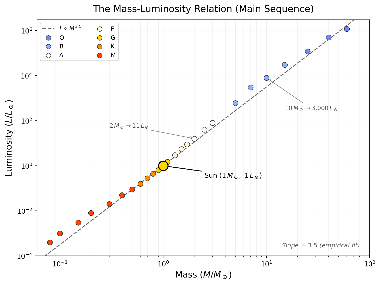
Main-sequence stars fall on a remarkably tight power law. The scatter everyone expected simply isn’t there.
~44–45 min. Point to the log-log plot. “Each point is a star with a dynamically measured mass from a binary system. The trend is unmistakable. Point to the Sun at (1,1). Point to the steep slope.”
Real Measurements: Binary Star Data
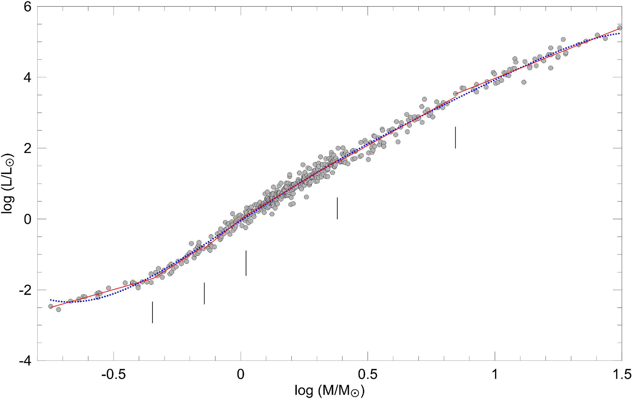
The scatter is real — composition, age, evolutionary state all contribute. But the trend is remarkably tight for astrophysics.
~45 min. Quick slide. “This is what real data look like — not a perfect line, but tight enough to be one of the most useful relations in stellar astronomy.”
The Mass-Luminosity Relation
\[ \frac{L}{L_\odot} \approx \left(\frac{M}{M_\odot}\right)^{3.5} \tag{4}\]
- Exponent \(3.5\) is approximate — steeper at high mass (\({\sim}4\)), shallower at low mass (\({\sim}2.3\))
- Applies to main-sequence stars only — not giants, not white dwarfs
- Scaling: Double the mass → \(2^{3.5} \approx 11\times\) the luminosity. Ten times the mass → \({\sim}3{,}000\times\)
- Unit check: Both sides are ratios (dimensionless). \(\checkmark\)
Applies only to main-sequence stars. Giants and white dwarfs do NOT follow this relation.
Luminosity depends on internal structure, not just total mass, once a star evolves.
~46 min. Establish the law, validity range, and scaling behavior.
The Mass-Luminosity Relation: Why So Steep?
Why so steep?
- Higher mass → higher central pressure
- Higher temperature → nuclear reaction rates increase rapidly
- Nuclear energy generation rates scale roughly as \(\epsilon \propto T^n\), where \(n \gg 1\)
- Small temperature increase → large luminosity increase
The prediction answer: \(L(2\,M_\odot) = 2^{3.5} \approx 11\,L_\odot\) — not \(2\times\), not \(4\times\), but \(11\times\)!
The universe is fiercely nonlinear.
~46–47 min. Reveal the answer to the prediction. “Most of you guessed (a) or (b). A factor of 2 in mass gives a factor of 11 in luminosity. This is wildly steeper than linear.”
Small Mass Changes, Huge Consequences
| Mass (\(M_\odot\)) | \(L/L_\odot \approx (M/M_\odot)^{3.5}\) | Factor relative to Sun |
|---|---|---|
| \(0.1\) | \(0.1^{3.5} = 3.2 \times 10^{-4}\) | \(3 \times 10^3\!\times\) fainter |
| \(0.5\) | \(0.5^{3.5} = 0.088\) | \(11\times\) fainter |
| \(1.0\) | \(1.0\) | \(1\times\) (the Sun) |
| \(2.0\) | \(2.0^{3.5} = 11.3\) | \(11\times\) brighter |
| \(10\) | \(10^{3.5} = 3.2 \times 10^3\) | \({\sim}3 \times 10^3\!\times\) brighter |
| \(50\) | \(50^{3.5} = 8.8 \times 10^5\) | \({\sim}10^6\!\times\) brighter |
Mass range: \({\sim}10^3\!\times\). Luminosity range: \({\sim}10^{10}\!\times\).
~47 min. Walk through a few rows. “Factor of 2,000 in mass produces a factor of 10 billion in luminosity. Let that number land.”
Massive Stars Live Fast & Die Young
For main-sequence stars, the fuel is core hydrogen, and available hydrogen fuel scales with mass \(M\). Its burn rate scales with luminosity:
\[ L \propto M^{3.5} \]
So:
\[ \begin{aligned} t_{\text{MS}} &\sim \frac{\text{fuel}}{\text{burn rate}} \\ &\sim \frac{M}{L} \\ &\propto \frac{M}{M^{3.5}} = M^{-2.5} \end{aligned} \]
. . .
- Sun: \(t_\odot \sim 10~\text{Gyr}\)
- \(10\,M_\odot\) star: \(t \sim 10 \times 10^{-2.5}~\text{Gyr} \approx 30~\text{Myr}\) — roughly \(300\times\) shorter
- \(0.5\,M_\odot\) star: \(t \sim 10 \times 0.5^{-2.5}~\text{Gyr} \approx 57~\text{Gyr}\)
~48 min. “The derivation is beautiful in its simplicity: fuel over burn rate. More mass means more fuel, but the burn rate grows far faster. The result: massive stars live fast and die young.”
Main-Sequence Lifetime Cutoff
The universe is \(13.8~\text{Gyr}\) old.
. . .
Using \(t_{\text{MS}} \sim 10~\text{Gyr}\,\left(\frac{M}{M_\odot}\right)^{-2.5}\) and setting \(t_{\text{MS}} = 13.8~\text{Gyr}\):
\[ 13.8~\text{Gyr} \sim 10~\text{Gyr}\left(\frac{M_{\text{cut}}}{M_\odot}\right)^{-2.5} \]
\[ \frac{13.8~\text{Gyr}}{10~\text{Gyr}} \sim \left(\frac{M_{\text{cut}}}{M_\odot}\right)^{-2.5} \quad\Rightarrow\quad \frac{M_{\text{cut}}}{M_\odot} \sim \left(\frac{10~\text{Gyr}}{13.8~\text{Gyr}}\right)^{1/2.5} \]
\[ \frac{10~\text{Gyr}}{13.8~\text{Gyr}} = 0.725,\quad \frac{M_{\text{cut}}}{M_\odot} \approx 0.88 \]
So \(M_{\text{cut}} \approx 0.88\,M_\odot\).
. . .
So, in this scaling estimate:
- Stars with \(M \lesssim 0.9\,M_\odot\) can still be on the main sequence today
- A \(0.5\,M_\odot\) star (\(t_{\text{MS}} \sim 57~\text{Gyr}\)) is safely below that cutoff
- Stars above this mass can already have exhausted core hydrogen
~49 min. Emphasize this is an estimate from the main-sequence scaling relation, not a sharp boundary. The key idea: there is a mass threshold set by the universe’s age, around \(0.9\,M_\odot\).
Quick Check: Scaling
A \(3\,M_\odot\) main-sequence star has luminosity approximately:
- \(3\,L_\odot\)
- \(9\,L_\odot\)
- \(27\,L_\odot\)
- \({\sim}47\,L_\odot\)
~50 min. Give 30 seconds. Press C to reveal. Walk through the exponentiation: \(3^3 = 27\), \(3^{0.5} \approx 1.73\), product \(\approx 47\). “This is the kind of mental math you should be practicing — split \(3.5 = 3 + 0.5\) and multiply.”
Quick Check Debrief: Scaling
\[ \frac{L}{L_\odot} = \left(\frac{M}{M_\odot}\right)^{3.5} = \left(\frac{3\,M_\odot}{M_\odot}\right)^{3.5} = 3^{3.5} = 3^3 \times 3^{0.5} = 27 \times 1.73 \approx 47 \]
So \(L \approx 47\,L_\odot\).
~50–51 min. Reveal after the vote. Keep this brisk and emphasize the unit ratio form first.
Mass Determines Everything
- Luminosity follows from mass
- Temperature follows from mass (through stellar structure)
- Radius follows from \(L\) and \(T\): Stefan-Boltzmann
- Lifetime follows from mass: \(t \propto M^{-2.5}\)
- Death follows from mass: low mass → white dwarf; high mass → supernova → neutron star or black hole
\[ L \propto M^{3.5} \]
Measure the mass — the life story follows.
Mass Detective — Case Closed. The suspect has been identified: mass is the master variable. It controls everything.
~51 min. This is the payoff slide. “One number — mass — controls the entire life story of a star. Its luminosity, temperature, radius, how long it lives, how it dies. This is why the mass-luminosity relation is the single most important empirical relation in stellar astrophysics.”
Observable → Model → Inference
Observable: Periodic Doppler shifts in spectral lines (and eclipses, when present)
Model: Two stars orbiting a common center of mass under Newtonian gravity
Inference: From \((P, K_1, K_2) \rightarrow (M_1, M_2)\) From many binaries:
\[ L \propto M^{3.5} \]
~52 min. Explicit O→M→I frame. “From wavelength oscillations in a spectrograph, we infer the most important property of stars. That’s the power of physics applied to observation.”
The Module 2 Inference Chain — Complete
| Lecture | Tool | Question Answered | What It Unlocks |
|---|---|---|---|
| 1 | Parallax → distance | How far? | Distance \(d\); then \(L = 4\pi d^2 F\) |
| 2 | Color/flux → temperature; Stefan-Boltzmann | How hot? How big? | Temperature \(T\); radius \(R\) |
| 3 | Spectral lines → composition, Doppler | What’s it made of? How is it moving? | Composition; velocity \(v_r\) |
| 4 | Binary orbits → mass | How heavy? | Mass \(M\); mass-luminosity relation |
From photons alone: distance, luminosity, temperature, radius, composition, and mass.
~53 min. “Four lectures, six fundamental properties, all extracted from light. The toolkit is complete. Next: we put all these measurements on one diagram and see what patterns emerge.”
Summary: Key Takeaways
- Mass is the master variable — determines luminosity, temperature, radius, lifetime, and death — but cannot be measured from a single star’s light alone
- Binary stars reveal masses — visual (orbits on sky), spectroscopic (Doppler velocities), eclipsing (inclination + radii)
- Newton’s Kepler III for binaries gives total mass; center-of-mass physics gives the mass ratio
- Mass-luminosity relation — the most important empirical scaling connecting mass to luminosity
- Lifetime scales as \(M^{-2.5}\) — massive stars die young; low-mass stars are nearly eternal
~54 min. Read through once. Each takeaway maps to a learning objective.
The Takeaway
If you forget everything else from today, remember this:
Measure the mass — the life story follows.
Mass determines a star’s luminosity, lifetime, and death — and binary stars are the only way to measure it.
~55 min. Let this land. This is the single-sentence summary of Lecture 4.
Questions?
- “Can we measure mass for stars not in binaries?” — Only indirectly, through model-dependent methods like spectroscopic parallax + mass-luminosity relation
- “What about triple or quadruple systems?” — They exist! Same physics, harder analysis
- “Why doesn’t the mass-luminosity relation work for giants?” — Giants have evolved off the main sequence; their luminosity depends on evolutionary state, not just current mass
The main sequence is a mass sequence.
~56 min. Address anticipated questions. Save time for actual student questions.
Next Time: The HR Diagram
Lecture 5: We assemble all measurements onto one diagram.
- Plot luminosity vs. temperature for thousands of stars
- The main sequence, red giants, white dwarfs — striking patterns emerge
- The main sequence turns out to be a mass sequence — thanks to what you learned today
The patterns demand a physical explanation. Module 3 will provide it.
Binaries calibrate the mass–luminosity relation, which lets us interpret the main sequence physically.
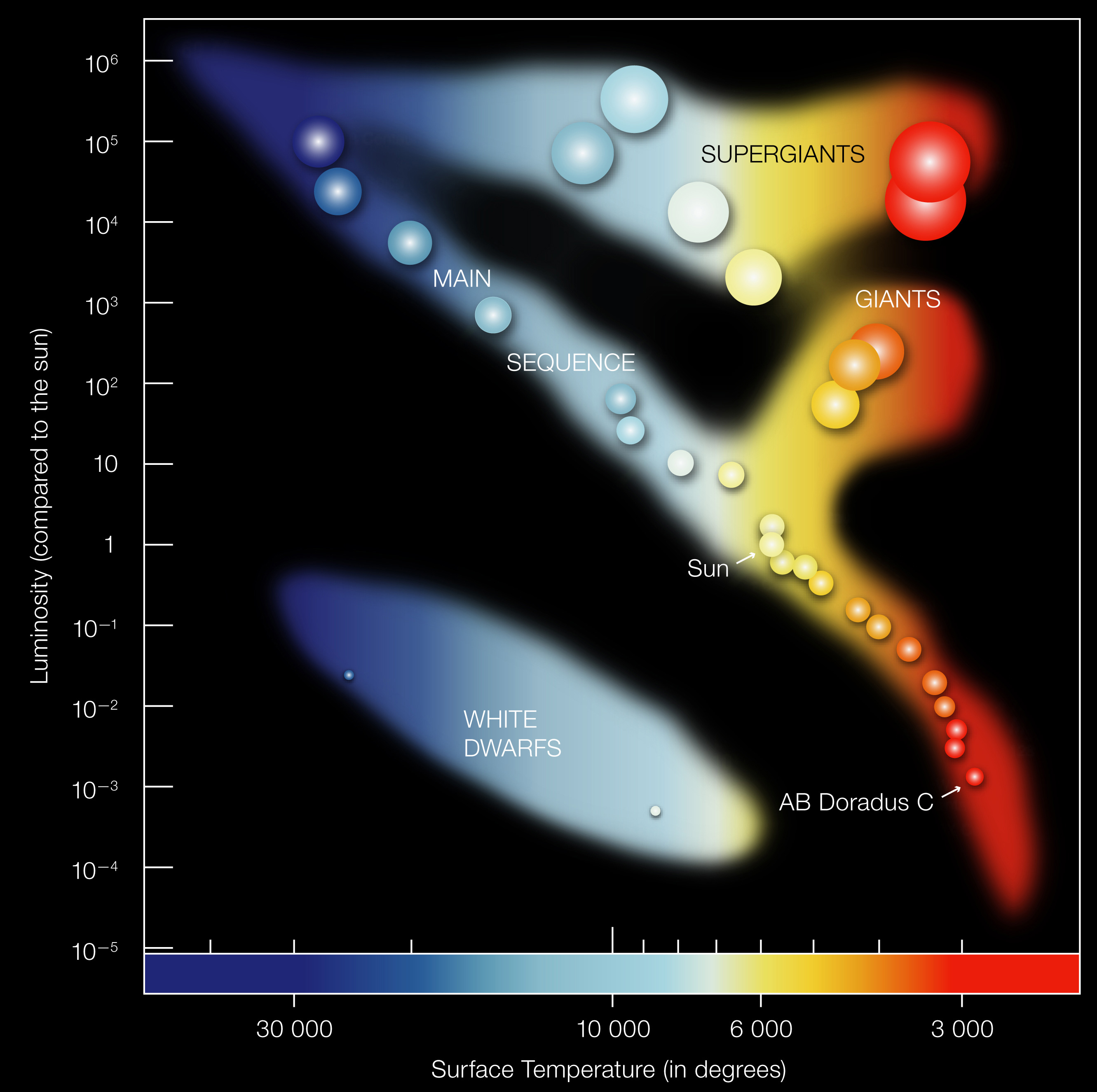
Preview: the HR diagram plot we will unpack next lecture.
~57 min. Build anticipation. “Today you learned that mass controls everything. Next time, we’ll see it — plotted on a single, powerful diagram. And the patterns that emerge will drive the rest of the course.”