The HR Diagram

Finding Patterns, Needing Models

Dr. Anna Rosen

February 26, 2026

Learning Objectives

1. Define apparent and absolute magnitude and apply the distance modulus formula
2. Convert between magnitude differences and flux ratios using the Pogson relation
3. Construct the observer’s HR diagram (\(M_V\) vs. spectral type) and identify its major features
4. Construct the theorist’s HR diagram (\(\log L\) vs. \(\log T_{\text{eff}}\)) and derive lines of constant radius
5. Identify the main sequence, giant branch, and white dwarf sequence
6. Explain why the main sequence is a mass sequence
7. Articulate the questions the HR diagram raises — and why physics (Module 3) is needed to answer them

~1 min. Read aloud. Seven objectives — more than usual because this lecture covers the magnitude system AND the HR diagram. These map to the seven summary points at the end.

They expected scatter.

They found structure.

The question today is not what the HR diagram looks like — it’s why the universe prefers order over randomness.

0–1 min. Let this sit for 5 seconds. “When Hertzsprung and Russell plotted luminosity against temperature for hundreds of stars, they expected a random spray — every star is different, after all. Instead, they found highways, clusters, sequences. That pattern is one of the most important discoveries in all of astrophysics.”

Today’s Roadmap

1. The Magnitude System — the astronomer’s logarithmic brightness scale
2. The Observer’s HR Diagram — patterns from data alone
3. The Theorist’s HR Diagram — overlaying physics (lines of constant radius)
4. Mass: The Hidden Organizer — why the main sequence is a mass sequence
5. An Evolution Diagram — stars move, and the patterns demand physics (→ Module 3)

~1–2 min. Quick orientation. “Today is the culmination of Module 2. We add one last measurement tool — magnitudes — then assemble everything onto one diagram. The patterns we find will drive the rest of the course.”

Map Builder

We’re building a map of the stars. By the end, every star has an address — and mass writes the zip code.

~2–3 min. Introduce the running motif. “Think of today as map-building. We start with blank axes, populate them with data, and watch structure emerge. Each section adds a layer — measurement, structure, physics, mass, time.”

The Magnitude System

The astronomer’s brightness scale

~3 min. Section divider. “Before we can build the HR diagram, we need one more tool: a way to compare stellar brightnesses across an enormous range.”

Stars Span a Ridiculous Range

• Betelgeuse delivers \(6 \times 10^7\!\times\) more flux than Proxima Centauri
• The Sun delivers \(6 \times 10^{10}\!\times\) more flux than Betelgeuse (because it’s close)
• Total range: more than \(10^{10}\) — a linear scale is useless

You need a logarithmic scale. That scale is the magnitude system — where multiplicative flux changes become additive magnitude shifts.

~3–4 min. “If you plotted all three on a linear chart, two would be invisible dots at zero. You need a scale that compresses ten orders of magnitude into manageable numbers. Astronomers have one — and it comes with a 2,000-year-old quirk.”

The Backward Scale

Brighter objects have smaller (more negative) magnitudes.

Object	Apparent magnitude \(m\)
Sun	\(-26.74\)
Sirius	\(-1.46\)
Vega	\(+0.03\)
Naked-eye limit	\({\sim}+6\)
Hubble limit	\({\sim}+31\)

Hipparchus (2nd century BCE): “first magnitude” = brightest. Modern astronomy formalized this — but kept the backward convention.

~4–5 min. “There’s no deep reason — it’s a historical accident that stuck. But it’s universal, so you must internalize it. Brighter means smaller. Say it with me: brighter means smaller.”

Why Logarithms? A 60-Second Refresher

The magnitude system is built on \(\log_{10}\). Three properties do all the work:

Property	Rule	Example
Product → Sum	\(\log(A \times B) = \log A + \log B\)	\(\log(100 \times 1{,}000) = 2 + 3 = 5\)
Ratio → Difference	\(\log(A / B) = \log A - \log B\)	\(\log(1{,}000 / 10) = 3 - 1 = 2\)
Power → Multiply	\(\log(A^n) = n \log A\)	\(\log(10^{3.6}) = 3.6\)

Why this matters: Magnitudes use \(\log_{10}(\text{flux ratio})\). The distance modulus uses \(\log_{10}(d)\). The HR diagram uses \(\log L\) and \(\log T\). Logarithms turn multiplicative relationships into additive ones — multiplication becomes addition.

~5 min. Quick refresher — most students have seen these rules but may not have used them recently. “If logs are rusty, memorize three rules: products become sums, ratios become differences, powers become multipliers. That’s all you need for the rest of today.”

Optional: 20-Second Log Refresher

• Product: \(\log(AB)=\log A+\log B\)
• Ratio: \(\log(A/B)=\log A-\log B\)
• Power: \(\log(A^n)=n\log A\)
• Anchor: \(\log_{10}(2)\approx 0.3\)

Logarithms in Action: Key Values

\(x\)	\(\log_{10} x\)	How to remember
\(1\)	\(0\)	\(10^0 = 1\)
\(10\)	\(1\)	Definition
\(100\)	\(2\)	\(10^2\)
\(1{,}000\)	\(3\)	\(10^3\)
\(2\)	\(0.301\)	\(\approx 0.3\) (useful!)
\(3\)	\(0.477\)	\(\approx 0.5\)
\(0.1\)	\(-1\)	\(10^{-1}\)
\(0.01\)	\(-2\)	\(10^{-2}\)

Mental math: \(\log_{10}(200) = \log(2 \times 100) = 0.3 + 2 = 2.3\). That’s how we’ll estimate distances from magnitudes.

~5–6 min. “Knowing \(\log 2 \approx 0.3\) and \(\log 3 \approx 0.5\) lets you estimate almost anything. We’ll use this constantly — in the distance modulus, on the HR diagram axes, everywhere.”

Apparent Magnitude: The Pogson Relation

\[ m_1 - m_2 = -2.5\,\log_{10}\!\left(\frac{F_1}{F_2}\right) \tag{1}\]

• \(m_1, m_2\) = apparent magnitudes of two sources
• \(F_1, F_2\) = fluxes (energy per unit area per unit time)
• Scaling: Each \(1~\text{mag}\) difference = factor of \(10^{0.4} \approx 2.512\) in flux
• Unit check: Flux ratio is dimensionless; magnitude difference is dimensionless. \(\checkmark\)

Anchor: 5 magnitudes = exactly a factor of 100 in flux (by definition).

~5–7 min. Unpack carefully. “The 2.5 and the log₁₀ combine so that 5 magnitudes equals exactly 100× in flux. That’s the one number to memorize — everything else follows.”

Magnitude–Flux Conversion: Key Numbers

Magnitude difference \(\Delta m\)	Flux ratio \(F_1/F_2\)
\(1~\text{mag}\)	\(10^{0.4} \approx 2.512\)
\(2~\text{mag}\)	\(10^{0.8} \approx 6.31\)
\(5~\text{mag}\)	\(10^{2.0} = 100\)
\(10~\text{mag}\)	\(10^{4.0} = 10{,}000\)
\(15~\text{mag}\)	\(10^{6.0} = 10^6\)

Mental math trick: \(\Delta m = 5\) → \(\times 100\). Double it: \(\Delta m = 10\) → \(\times 10{,}000\). Add 5 more: \(\Delta m = 15\) → \(\times 10^6\).

~7–8 min. “You don’t need the whole table. Just remember 5 mag = 100×. Then 10 mag = 100² = 10,000. And 15 mag = 100³ = a million. That’s how astronomers do mental math with magnitudes.”

Quick Check: Flux Ratio

Star X has \(m = 3.0\) and Star Y has \(m = 8.0\). How many times brighter is Star X?

• \(5\times\) — magnitude difference equals flux ratio
• \(25\times\) — square of the magnitude difference
• \(100\times\) — since \(\Delta m = 5.0\) and \(5~\text{mag} = 100\times\)
• \(10{,}000\times\) — that would require \(\Delta m = 10\)

~8–9 min. Give 20 seconds. Press C to reveal. \(\Delta m = 8.0 - 3.0 = 5.0~\text{mag}\). Five magnitudes = exactly \(100\times\) in flux. Sanity check: Star X has a smaller (brighter) magnitude, so it is indeed brighter. \(\checkmark\)

Absolute Magnitude: A Fair Comparison

• Apparent magnitude \(m\) mixes intrinsic brightness with distance
• A nearby dim star can look brighter than a distant luminous one
• To compare stars fairly: place them all at the same distance

Absolute magnitude \(M\) = the apparent magnitude a star would have at a standard distance of \(10~\text{pc}\).

This measures intrinsic brightness — the star’s luminosity in the magnitude system.

~9–10 min. “Apparent magnitude tells you how bright a star looks. Absolute magnitude tells you how bright it is. The difference is distance — and we need the distance modulus to connect them.”

Apparent vs. Absolute: Four Stars

Star	\(m\) (apparent)	Distance	\(M\) (absolute)	\(L/L_\odot\)
Sun	\(-26.74\)	\(5 \times 10^{-6}~\text{pc}\)	\(+4.83\)	\(1\)
Sirius	\(-1.46\)	\(2.64~\text{pc}\)	\(+1.42\)	\(25\)
Betelgeuse	\(+0.42\)	\(200~\text{pc}\)	\(-5.85\)	\({\sim}10^5\)
Proxima Cen	\(+11.13\)	\(1.30~\text{pc}\)	\(+15.53\)	\(0.0017\)

The Sun looks blindingly bright (\(m = -26.74\)) only because it’s absurdly close. At \(10~\text{pc}\), it would be \(M = +4.83\) — visible but unremarkable.

~10–11 min. “Betelgeuse looks dim (\(m = +0.42\)) despite being \(10^5\) times more luminous than the Sun — it’s 200 pc away. This is exactly why we need absolute magnitude.”

The Distance Modulus

\[ m - M = 5\log_{10}\!\left(\frac{d}{10\,\mathrm{pc}}\right) \tag{2}\]

• \(m\) = apparent magnitude (observed)
• \(M\) = absolute magnitude (intrinsic)
• \(d\) = distance in parsecs
• \((m - M)\) = the distance modulus
• Scaling: Every \(5~\text{mag}\) increase in \((m-M)\) = \(10\times\) farther
• What it is: The inverse-square law (\(F = L/4\pi d^2\)) rewritten in the astronomer’s logarithmic language

~11–12 min. “This is NOT a new equation — it’s the inverse-square law you already know from Lecture 1, just re-packaged in magnitudes. The \(d^2\) dependence of flux becomes a \(5\log_{10}(d)\) dependence in magnitudes.”

Distance Modulus: Sanity Checks

• At \(d = 10~\text{pc}\): \(m - M = 5\log_{10}(10/10) = 0\) → \(m = M\). \(\checkmark\) (Definition of \(M\).)
• At \(d = 100~\text{pc}\): \(m - M = 5\log_{10}(100/10) = 5\). Star appears \(5~\text{mag}\) (\(100\times\)) fainter. \(\checkmark\)
• At \(d = 1{,}000~\text{pc}\): \(m - M = 10\). Star is \(10^4\!\times\) fainter. \(\checkmark\)

Pattern: Each factor of \(10\) in distance adds \(5~\text{mag}\) to the distance modulus.

~12–13 min. Walk through each. “The first is just the definition — at 10 pc, apparent equals absolute. The pattern is clean: factor of 10 in distance = 5 more magnitudes.”

Worked Example: How Far Is This Cepheid?

Problem: A Cepheid variable has \(m = 14.0\) and (from its pulsation period) \(M = -4.0\). Find \(d\).

Step 1 — Distance modulus: \(m - M = 14.0 - (-4.0) = 18.0~\text{mag}\)

Step 2 — Solve for distance:

\[\log_{10}\!\left(\frac{d}{10~\text{pc}}\right) = \frac{18.0}{5} = 3.6 \quad \Rightarrow \quad d = 10^{3.6} \times 10~\text{pc} \approx 4.0 \times 10^4~\text{pc} = 40~\text{kpc}\]

Sanity check: \(40~\text{kpc}\) is comparable to the Milky Way’s diameter — reasonable for a luminous Cepheid (\(M = -4.0\) means \(L \sim 5{,}000\,L_\odot\)). \(\checkmark\)

~13–15 min. Walk through with pauses. “The distance modulus of 18 is large — \(10^{3.6} \approx 4{,}000\) times the standard 10 pc. This puts the Cepheid at 40 kpc — the edge of the Galaxy.”

Quick Check: Distance Modulus

A star has apparent magnitude \(m = 5.0\) and absolute magnitude \(M = 5.0\). How far away is it?

• \(1~\text{pc}\)
• \(10~\text{pc}\) — by definition, \(m = M\) means the star is at \(10~\text{pc}\)
• \(100~\text{pc}\)
• Cannot determine without luminosity

~15–16 min. Give 20 seconds. Press C to reveal. \(m - M = 0 = 5\log_{10}(d/10)\). So \(d/10 = 10^0 = 1\), giving \(d = 10~\text{pc}\). “This is just the definition of absolute magnitude — if \(m = M\), the star IS at 10 pc.”

Synthesis Check: Luminosity vs Distance

Star A is \(100\times\) more luminous than Star B, but Star A is also \(10\times\) farther away.

How do their apparent magnitudes compare?

• Star A appears \(5~\text{mag}\) brighter
• They appear equally bright (\(\Delta m = 0\)) — flux scales as \(L/d^2\), so \(100/(10^2)=1\)
• Star A appears \(5~\text{mag}\) fainter
• Cannot determine without spectral type

~16 min. Give 20–30 seconds. This is the integration checkpoint before the HR diagram: inverse-square scaling plus magnitude intuition in one step.

The Observer’s HR Diagram

Patterns from data alone

~16 min. Section divider. “You now have both axes: absolute magnitude and spectral type. No theory needed — pure measurement. Let’s plot and see what emerges.”

A Radical Idea: Plot Everything

By the early 1900s, astronomers had spectral types and parallax distances for thousands of stars.

Ejnar Hertzsprung (Denmark, 1911) and Henry Norris Russell (Princeton, 1913) independently asked: what happens if you plot absolute magnitude against spectral type?

Every star has different mass, age, and composition. The natural expectation: noise — a random spray of dots.

What they found instead was one of the most stunning patterns in all of science.

~17–18 min. Build the tension. “They had no theoretical reason to expect anything other than scatter. Every star is different — why should there be a pattern? But when they plotted the data…” [transition to next slide]

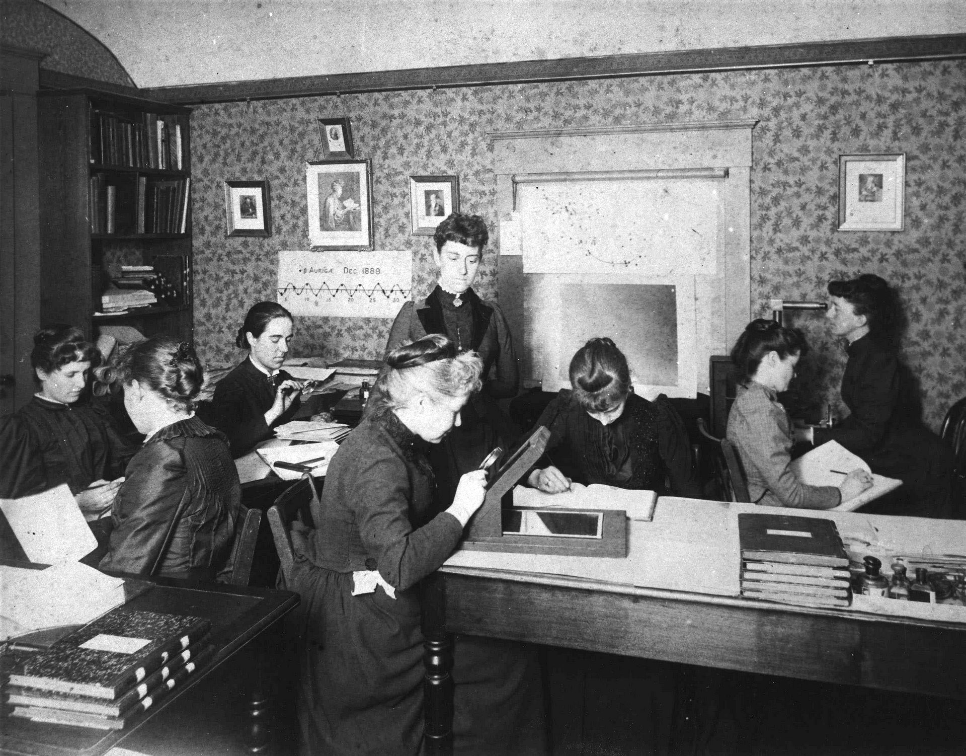
Cecilia Payne-Gaposchkin: Decoding the Diagram

Credit: Harvard College Observatory / Smithsonian Institution

• 1925 PhD thesis (age 25): Connected the HR diagram’s axes to physics
• The horizontal axis is a temperature sequence, not a composition sequence
• All stars are overwhelmingly hydrogen and helium
• Struve: “undoubtedly the most brilliant PhD thesis ever written in astronomy”

~18–19 min. “The Harvard Computers built OBAFGKM. Payne decoded what it means. The spectral sequence is a temperature sequence — hot O stars on the left, cool M stars on the right. The chemistry is the same; only the temperature changes.”

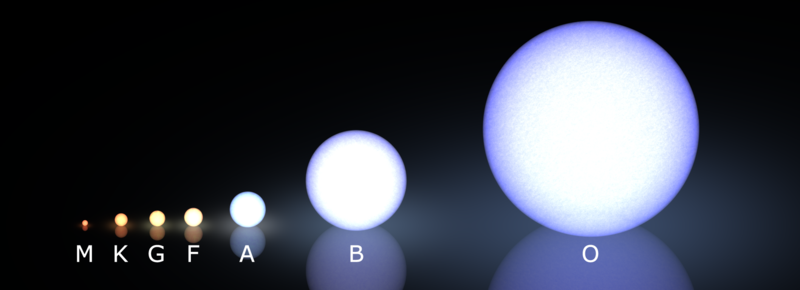
The Horizontal Axis: OBAFGKM Revisited

Credit: NOAO/AURA/NSF

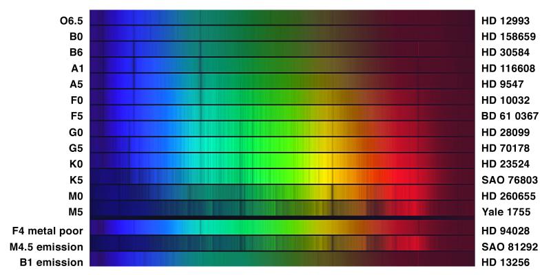
From Lecture 3: the spectral sequence is a temperature sequence.

• O → hot (\(> 30{,}000~\text{K}\)), blue
• M → cool (\({\sim}3{,}000~\text{K}\)), red
• Line strengths trace \(T\), not composition
• This sequence becomes the HR diagram’s horizontal axis

~18–19 min. Lecture 3 callback. “Remember the spectral sequence? Payne showed it’s temperature-ordered. Now that sequence becomes the horizontal axis of the most important diagram in stellar astrophysics.”

The Observer’s HR Diagram

Credit: ASTR 201 (generated)

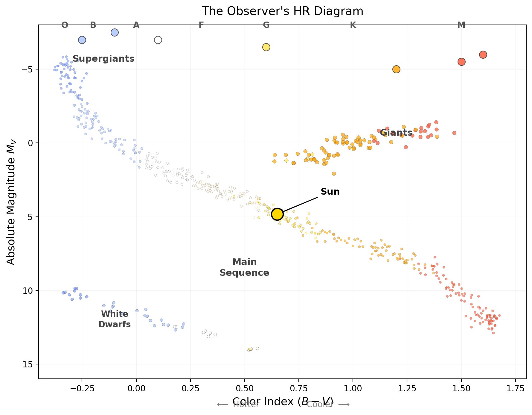
Axes (both backwards!):

• Vertical: \(M_V\) — brighter (more negative) at top
• Horizontal: spectral type — hotter on the left, cooler on the right

Neither axis requires theory — this is pure measurement.

Three structures jump out immediately.

~19–20 min. Point to the diagram. “The vertical axis goes backward — more negative (brighter) at top. The horizontal axis also goes backward — hotter at left. Both conventions are historical, but universal. Now look at the data.”

Axis Anchor (Do Not Forget)

Hotter \(\leftarrow\)

Brighter \(\uparrow\)

Every confusion about the HR diagram starts with forgetting one of these arrows.

~20 min. Make students say the arrows out loud: “Hotter left. Brighter up.”

Watch: Building an HR Diagram from Cluster Data

What to notice: a cluster’s stars do not land randomly. The main sequence, giant branch, and turnoff structure emerge from data and then demand a physical model.

~20–21 min. 45–60 second clip. “This is the measurement pipeline in motion: many stars, one system, one age, one composition trend, and a coherent HR pattern. The turnoff is the age clock.”

Predict: Name the Structures

Look at the HR diagram. Stars are NOT randomly scattered — they cluster into distinct regions.

(a) Where do most stars fall? What shape is that region?

(b) What’s unusual about the stars in the upper right? (Cool but luminous — how?)

(c) What’s unusual about the stars in the lower left? (Hot but faint — how?)

Hint: think about Stefan-Boltzmann (\(L = 4\pi R^2 \sigma T^4\)).

~20–21 min. Give 30 seconds. Don’t reveal yet — let the next slides build the answer. Students should recall Stefan-Boltzmann from Lecture 2: cool + luminous requires enormous radius; hot + faint requires tiny radius.

The HR Diagram: Annotated View

Credit: ESO

The labeled regions are not arbitrary — each corresponds to a physical class of stars with distinct sizes, luminosities, and evolutionary states.

If stars were arbitrary collections of gas, there would be no reason for a narrow diagonal band to exist. Something is constraining their internal structure.

~21–22 min. “This annotated version shows the named regions explicitly. Main sequence dominates; giants and supergiants occupy the upper right; white dwarfs huddle in the lower left. Every region has a physical explanation.”

The Main Sequence

• A narrow diagonal band from upper-left (hot, bright) to lower-right (cool, faint)
• 90% of all stars fall on this band
• The Sun sits roughly in the middle (G2, \(M_V = +4.83\))

This is not a coincidence. From Lecture 4: mass determines luminosity (\(L \propto M^{3.5}\)) and temperature. The main sequence is a mass sequence — but that reveal comes in Part 4.

~22–23 min. “Ninety percent. Not a trend — a highway. And it turns out to be organized by a single hidden variable. We’ll get there.”

Giants and White Dwarfs

Upper Right: Giants

Cool (\(T \sim 3{,}000\text{–}5{,}000~\text{K}\)) but luminous (\(100\text{–}10^4\,L_\odot\)).

Stefan-Boltzmann demands enormous radii: \(R \sim 10\text{–}100\,R_\odot\).

A red giant’s photosphere could extend halfway to Mercury’s orbit.

Lower Left: White Dwarfs

Hot (\(T \sim 10^4\text{–}3 \times 10^4~\text{K}\)) but faint (\({\sim}0.01\,L_\odot\)).

Stefan-Boltzmann demands tiny radii: \(R \sim 0.01\,R_\odot\) — Earth-sized.

Dead stellar cores, no longer burning fuel.

~22–24 min. “Both extremes are explained by Stefan-Boltzmann. Cool but luminous? Must be huge. Hot but faint? Must be tiny. The physics you learned in Lecture 2 explains the geography.”

Think–Pair–Share: White Dwarf Radius

A star has \(T \sim 2.5 \times 10^4~\text{K}\) (about \(4\times\) hotter than the Sun) and \(L \sim 0.01\,L_\odot\).

1. Using \(L/L_\odot = (R/R_\odot)^2 (T/T_\odot)^4\), estimate \((R/R_\odot)^2\).
2. What familiar solar-system object has a similar radius?

30 seconds alone → 1 minute with a neighbor → share out

~24–26 min. TPS. Answer: \((R/R_\odot)^2 = 0.01/(4)^4 = 0.01/256 \approx 4 \times 10^{-5}\). So \(R/R_\odot \approx 0.006\). Earth is \(R_\oplus \approx 0.009\,R_\odot\) — so the white dwarf is roughly Earth-sized. “A stellar mass crammed into an Earth-sized volume. About a ton per teaspoon.”

Luminosity Classes: Vertical Structure

Even at the same spectral type, stars can differ enormously in luminosity. Spectral line widths reveal why — they encode surface gravity.

Class	Name	Surface gravity	Lines	Example
I	Supergiant	Low \(g\)	Narrow	Betelgeuse (M1 I)
III	Giant	Moderate	—	Arcturus (K1 III)
V	Main-seq dwarf	High \(g\)	Broad	Sun (G2 V)

Full classification = spectral type + luminosity class: G2 V (Sun), M1 I (Betelgeuse).

~26–27 min. “A K2 dwarf and a K2 giant have the same temperature but luminosities differing by 500×. Line widths tell them apart: high gravity broadens lines (compact dwarfs), low gravity keeps them narrow (extended giants). This is pressure broadening from Lecture 3.”

Quick Check: Stellar Classification

A star is classified as K5 III. Which statement is correct?

• It is hotter than the Sun and a main-sequence dwarf
• It is cooler than the Sun and a main-sequence dwarf
• It is cooler than the Sun and a giant — K is cooler than G; class III = giant
• It is hotter than the Sun and a giant

~27–28 min. Give 20 seconds. Press C to reveal. K is later (cooler) than G in the OBAFGKM sequence, so K5 is cooler than the Sun (G2). Class III = giant. “Two pieces of information in one label: temperature and luminosity class.”

Map Builder: Structures Identified

Three structures have emerged from the data.

• Main sequence — 90% of stars, a diagonal band ordered by temperature
• Giant branch — cool but luminous → enormous radii (\(10\text{–}100\,R_\odot\))
• White dwarfs — hot but faint → tiny radii (\({\sim}0.01\,R_\odot\))
• Luminosity classes add vertical structure: giants and dwarfs at the same temperature

The map has geography — but not yet physics. Let’s add it.

~28 min. Quick summary before transition. “We’ve identified the regions. But we haven’t explained them. The observer’s diagram is pure measurement. The theorist’s diagram adds physics.”

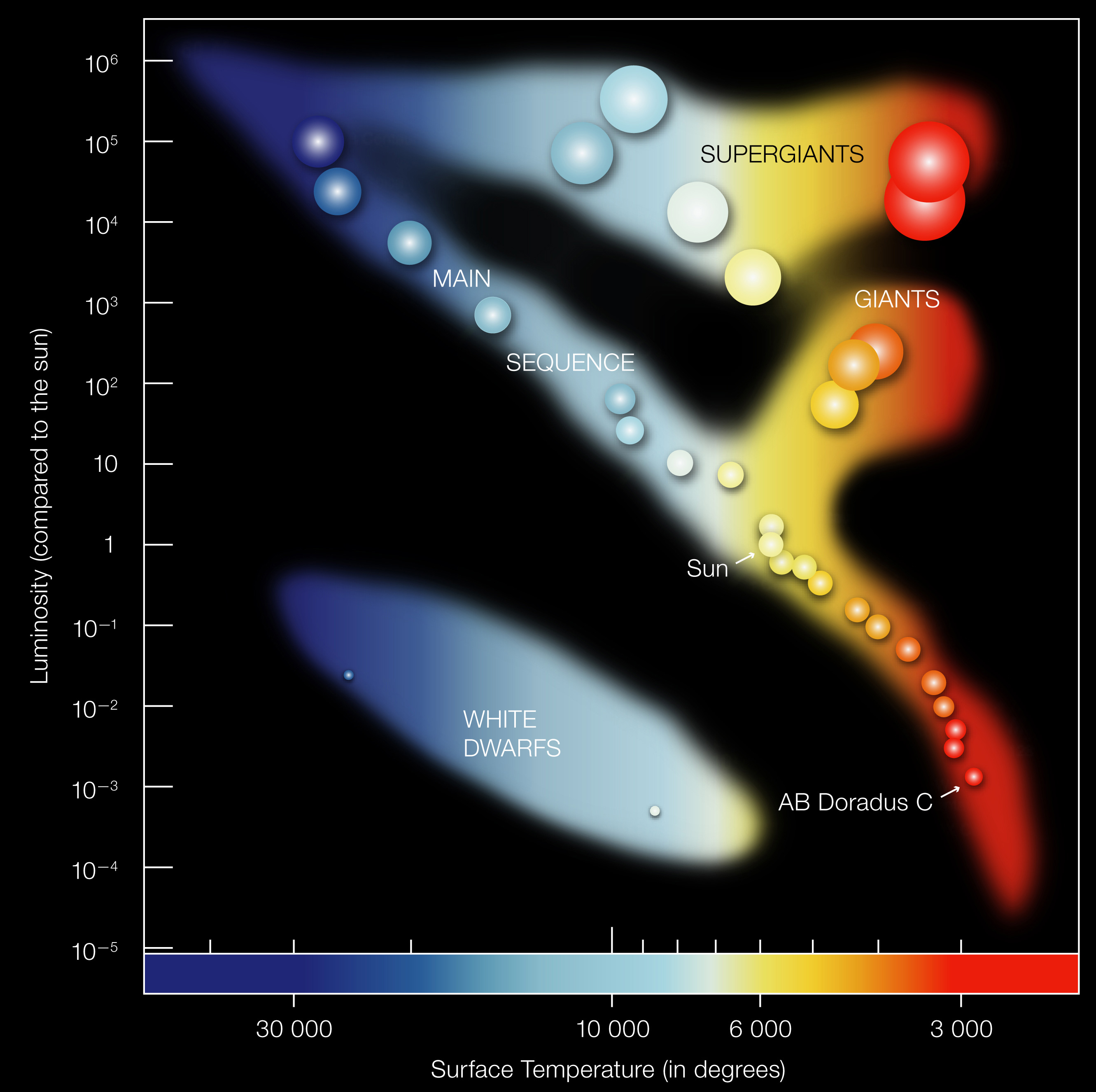
The Theorist’s HR Diagram

Overlaying physics on measurement

~28 min. Section divider. “Same data, different axes — and now we can overlay physical relationships.”

Same Patterns, Physical Axes

Observer’s diagram:

• \(M_V\) vs. spectral type
• Pure measurement
• No theory required

Theorist’s diagram:

• \(\log(L/L_\odot)\) vs. \(\log T_{\text{eff}}\)
• Physical quantities
• Can overlay theoretical relationships

The same patterns appear on both versions. The patterns are real features of stellar physics, not artifacts of the measurement system.

~29–30 min. “The observer’s axes are measured; the theorist’s axes are physical. But the patterns are identical — proving they’re real. Now the theorist’s version lets us add something the observer’s can’t: lines of constant radius.”

Stefan-Boltzmann → Lines of Constant Radius

From Lecture 2: \(L = 4\pi R^2 \sigma T^4\). On the HR diagram, \(L\) and \(T\) are the axes. Fix \(R\):

\[\log(L/L_\odot) = 2\log(R/R_\odot) + 4\log(T/T_\odot)\]

At fixed \(R\), this is a straight line with slope \(4\) on the \(\log L\) – \(\log T\) diagram.

Notice the steepness: at fixed radius, a \(0.1\) dex increase in \(\log T\) gives a \(0.4\) dex increase in \(\log L\).

• Scaling: Double \(T\) at fixed \(R\) → \(L\) increases by \(2^4 = 16\times\) (steep!)
• Shifting \(R\): Larger \(R\) moves the line up (brighter at every \(T\))
• Each line represents all possible \((L, T)\) combinations for a star of that radius
• These lines turn clustered points into constrained physical states

~30–32 min. Three reveals. “Stefan-Boltzmann connects three quantities. On the HR diagram, two are axes. Fixing the third — radius — draws a line. You can read a star’s radius from where it sits.”

The Theorist’s HR Diagram

Credit: ASTR 201 (generated)

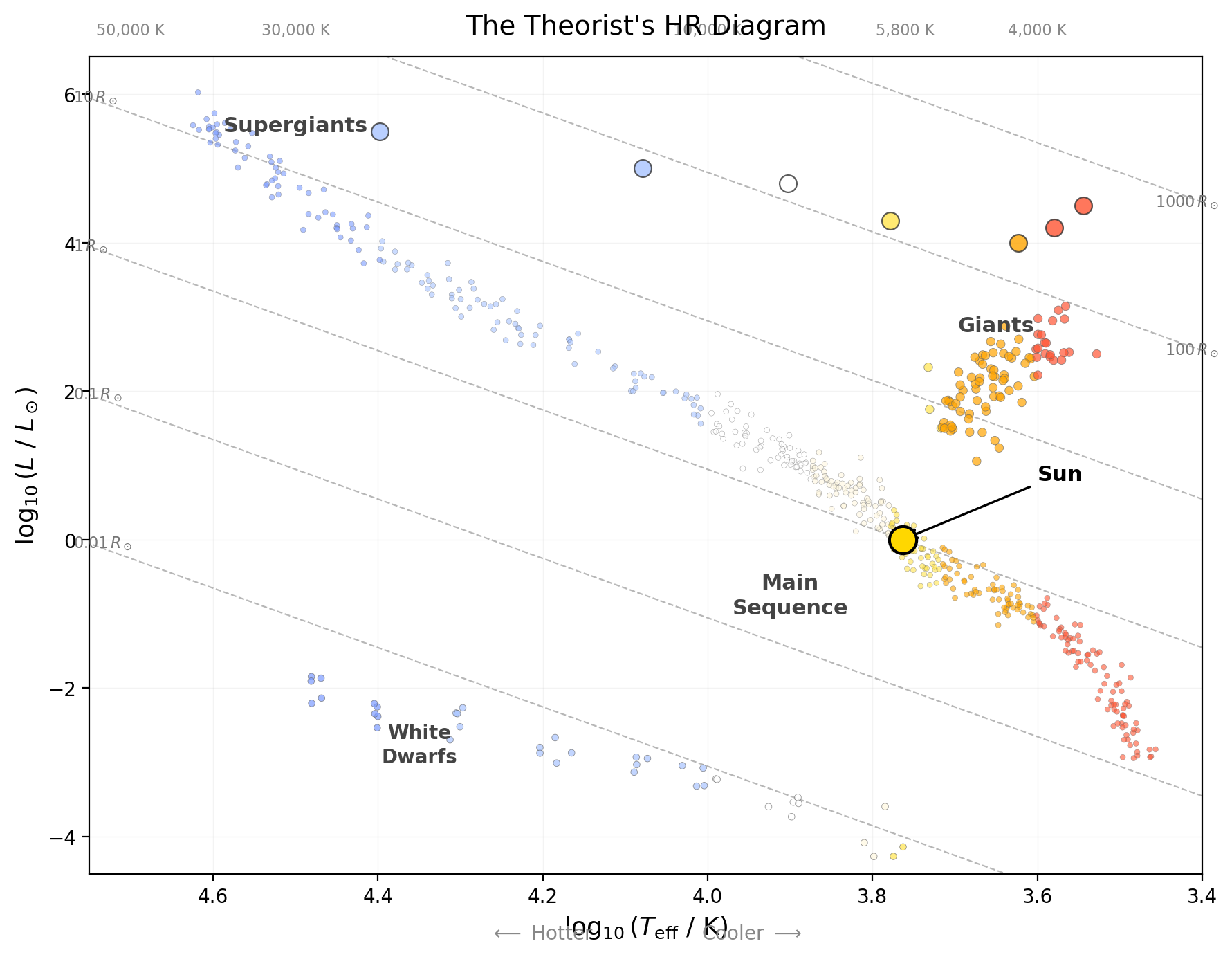
You can read radius directly from a star’s position. Three physical properties — \(L\), \(T\), \(R\) — encoded in a two-axis plot.

~32–33 min. Point to the radius lines. “Main-sequence stars: 0.1 to 10 solar radii. Giants: 10 to 100. Supergiants: 100 to 1,000. White dwarfs: 0.01 — Earth-sized.”

Reading Radius from Position

HR Region	Typical radius	Physical meaning
Main sequence	\(0.1\text{–}10\,R_\odot\)	Hydrogen-burning stars
Giants	\(10\text{–}100\,R_\odot\)	Evolved, expanded envelopes
Supergiants	\(100\text{–}1{,}000\,R_\odot\)	Most luminous evolved stars
White dwarfs	\({\sim}0.01\,R_\odot\)	Dead cores (Earth-sized)

Map Builder update: The map now has a size gradient — \(L\), \(T\), and \(R\) all readable from one diagram.

~33–34 min. “The radius range is staggering: from Earth-sized white dwarfs to supergiants bigger than Mars’s orbit. Stefan-Boltzmann encodes all of this.”

Size Along the Main Sequence

Credit: Wikimedia Commons (after Morgan & Keenan)

From O to M: luminosity spans \(10^{10}\), temperature spans a factor of \(14\), and radius spans a factor of \({\sim}100\). All driven by one hidden variable — mass.

~34–35 min. Point to the progression. “The physical size difference is dramatic — an O star could fit dozens of Suns inside it, while an M dwarf is barely bigger than Jupiter. This connects to the radius lines on the theorist’s diagram.”

Worked Example: Red Giant Radius

Problem: A red giant has \(L = 400\,L_\odot\) and \(T_{\text{eff}} = 4{,}000~\text{K}\). Find \(R/R_\odot\).

Ratio form (no constants needed!): \[\left(\frac{R}{R_\odot}\right)^2 = \frac{L/L_\odot}{(T/T_\odot)^4} = \frac{400}{(4{,}000/5{,}800)^4}\]

Temperature ratio: \(4{,}000/5{,}800 = 0.690\). Then \(0.690^4 = 0.226\).

\[\left(\frac{R}{R_\odot}\right)^2 = \frac{400}{0.226} = 1{,}770 \quad \Rightarrow \quad \frac{R}{R_\odot} = \sqrt{1{,}770} \approx 42\]

The red giant is \({\sim}42\,R_\odot\). Mercury orbits at \(0.39~\text{AU} \approx 84\,R_\odot\) — this star extends halfway there.

~34–36 min. “We used the ratio form — no CGS constants, no unit conversion. Just ratios. This is the scaling method from Lecture 2 applied to the HR diagram.”

Quick Check: White Dwarf Radius

A white dwarf has \(T_{\text{eff}} = 2 \times 10^4~\text{K}\) and \(L = 0.01\,L_\odot\). What is its radius?

• \({\sim}100\,R_\odot\) — a giant
• \({\sim}1\,R_\odot\) — Sun-sized
• \({\sim}0.1\,R_\odot\) — larger than a planet
• \({\sim}0.01\,R_\odot\) (Earth-sized) — since \((R/R_\odot)^2 = 0.01/(3.45)^4 \approx 7 \times 10^{-5}\)

~36–37 min. Give 30 seconds. Press C to reveal. \(T/T_\odot = 2 \times 10^4/5{,}800 = 3.45\). \((3.45)^4 \approx 142\). \((R/R_\odot)^2 = 0.01/142 = 7 \times 10^{-5}\). \(R/R_\odot \approx 0.008\). Earth is \(R_\oplus \approx 0.009\,R_\odot\). “Nearly a solar mass in an Earth-sized volume.”

Mass — The Hidden Organizer

The variable that doesn’t appear on either axis

~37 min. Section divider. “We’ve identified the structures, added physics, and read radii. But what organizes the main sequence? Why is there a highway at all?”

Predict: Mass Along the Main Sequence

From Lecture 4: more massive main-sequence stars are more luminous (\(L \propto M^{3.5}\)) and hotter.

If you labeled each main-sequence star with its mass, how would mass change along the sequence?

1. Mass increases randomly — no pattern

2. Mass increases from upper-left to lower-right

3. Mass increases from lower-right to upper-left — monotonically

Commit to an answer before the next slide.

~38 min. Give 20 seconds. Answer: (c). Mass increases monotonically from lower-right (cool, faint, low mass) to upper-left (hot, bright, high mass). “If \(L \propto M^{3.5}\), then more massive stars are more luminous — which direction is that on the diagram?”

The Main Sequence Is a Mass Sequence

Position	Type	\(M/M_\odot\)	\(L/L_\odot\)	\(T_{\text{eff}}\) (K)	Lifetime
Lower right	M5	\(0.1\)	\(0.001\)	\(3{,}000\)	\(> 100~\text{Gyr}\)
	M0	\(0.5\)	\(0.08\)	\(3{,}850\)	\({\sim}60~\text{Gyr}\)
Middle	G2 ☉	\(1.0\)	\(1.0\)	\(5{,}800\)	\({\sim}10~\text{Gyr}\)
	A0	\(2.5\)	\(40\)	\(9{,}900\)	\({\sim}1~\text{Gyr}\)
Upper left	B0	\(15\)	\(3 \times 10^4\)	\(3 \times 10^4\)	\({\sim}10~\text{Myr}\)
	O5	\(40\)	\(5 \times 10^5\)	\(4.2 \times 10^4\)	\({\sim}1~\text{Myr}\)

Mass increases monotonically from lower-right to upper-left. Mass — which does not appear on either axis — organizes the entire structure.

Nothing on the axes says “mass.” Yet mass organizes the entire pattern — the signature of a hidden variable.

~39–40 min. “A factor of 400 in mass produces a factor of \(5 \times 10^8\) in luminosity and a factor of \(10^5\) in lifetime. The main sequence is not a random band — it’s a mass sequence.”

The Mass-Luminosity Relation: Lecture 4 Callback

Credit: ASTR 201 (generated)

Credit: Eker et al. 2018, MNRAS 479, 5491

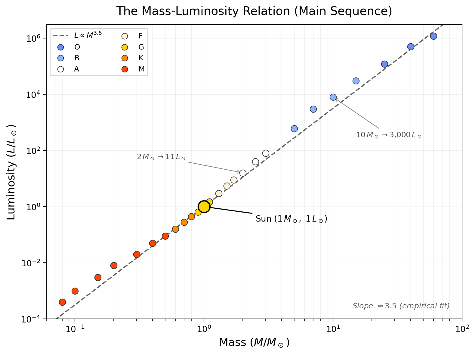
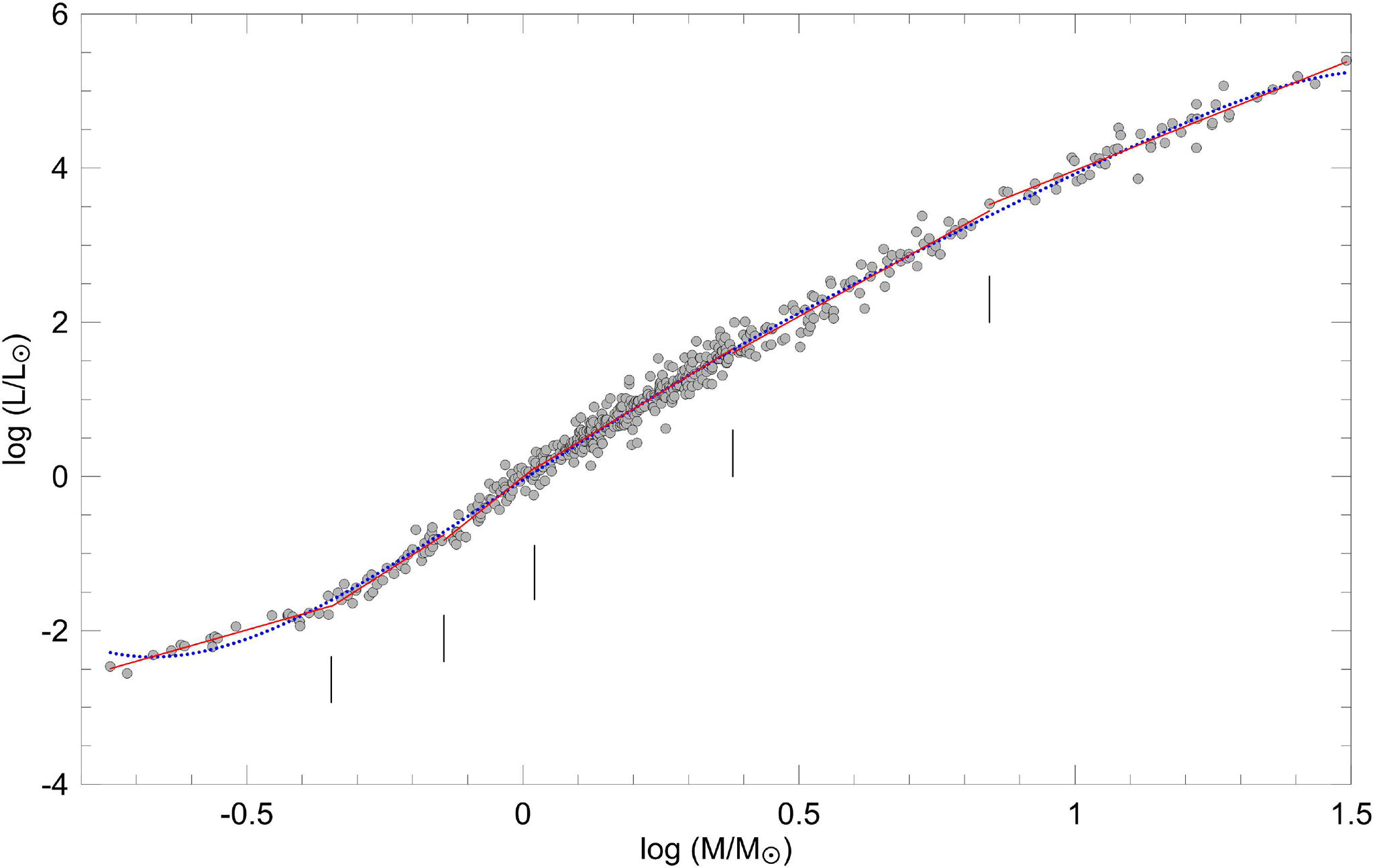
\(L \propto M^{3.5}\) explains the main sequence: mass sets core temperature → nuclear burning rate → luminosity and surface temperature. The scatter is real — but the trend is tight.

For main-sequence stars, this is an empirical scaling (not an exact law): the exponent varies with mass range and stellar structure, but the monotonic trend is robust.

~40–41 min. Quick callback. Left: idealized power law. Right: real binary-star measurements. “The scatter comes from metallicity differences, evolutionary state, and measurement uncertainty — but the power law is unmistakable.”

Spectroscopic Parallax: Distance from a Spectrum

• Every main-sequence star of a given mass has essentially the same \(L\) and \(T\)
• Know spectral type + luminosity class V → know \(M_V\) from the reference table
• Measure apparent magnitude \(m\) → distance modulus → distance

\[d = 10^{(m - M)/5 + 1}~\text{pc}\]

Distance from a spectrum — no parallax needed. This extends the distance ladder far beyond Lecture 1’s geometric parallax.

This works cleanly for main-sequence stars; giants and white dwarfs break the one-to-one spectral-type-to-luminosity mapping.

(Misnomer: nothing to do with parallax. But the name stuck.)

~41–42 min. “This closes the loop: Lecture 1 gave us parallax for nearby stars. Now the HR diagram extends distances to stars thousands of parsecs away — all from a spectrum and a magnitude.”

What About Giants and White Dwarfs?

• Giants/supergiants: Stars that have left the main sequence — exhausted core hydrogen, expanded dramatically. Position depends on mass + age + evolutionary state.
• White dwarfs: Remnants of dead stars — no longer burning fuel, just cooling. Position depends on mass + cooling time.

Main sequence = where stars live. Giants = where stars age. White dwarfs = where stars end up.

Map Builder: Mass writes the addresses — but the HR diagram is not a snapshot. It’s an evolution diagram.

~42–43 min. “Mass alone doesn’t organize giants and white dwarfs the way it organizes the main sequence. You need evolutionary state — and that brings us to Part 5.”

An Evolution Diagram

Why patterns need physics

~43 min. Section divider. “The HR diagram is not a snapshot. Stars move on it. Their path is determined by mass — and understanding that path requires the physics of stellar interiors.”

Stars Move on the HR Diagram

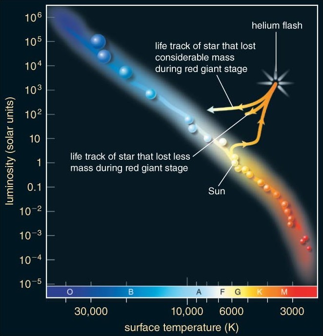
The life of a Sun-like star (\(1\,M_\odot\)), traced on the HR diagram:

1. Birth: Collapse from gas cloud → contracts toward the main sequence (upper right → middle)
2. Main sequence (\({\sim}10~\text{Gyr}\)): Hydrogen burning → stable equilibrium at (G2, \(1\,L_\odot\)) for \(10\) billion years
3. Red giant: Core hydrogen exhausted → core contracts, envelope expands → moves to upper right (\(R \sim 100\,R_\odot\))
4. Death: Sheds outer layers → white dwarf remnant in lower left, then slowly cools rightward

This motion is not random — it is the response of a self-gravitating system to changing fuel. 90% of stars are on the main sequence because that’s where they spend 90% of their lives.

~44–45 min. “Stars don’t wander randomly — each track is the response of gravity, thermodynamics, and nuclear burning acting together. When core hydrogen runs out, the core contracts, releasing gravitational energy that expands the envelope. The main sequence contains 90% of all stars because that’s where stars spend 90% of their time.”

Mass Sets the Pace of Evolution

High-mass stars peel away from the main sequence quickly; low-mass stars linger for billions of years. Same diagram, different clocks.

~45 min. Use this to bridge from “stars move” to “mass determines path and pace.” Point to short high-mass timescales vs long low-mass timescales.

Even Arrival to the Main Sequence Depends on Mass

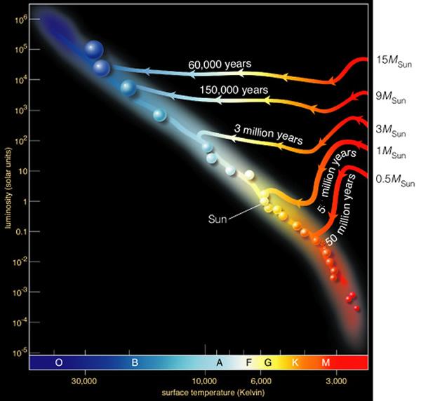
High-mass protostars reach the main sequence quickly; low-mass stars can spend tens of millions of years contracting toward it. Mass sets the evolutionary clock before stable fusion even begins.

~45 min. Optional enrichment if time. Use this only to reinforce that mass dependence starts before the main-sequence phase, not after it.

Mass Determines the Path

Low mass (\(0.5\,M_\odot\)):

• Slow, gentle evolution
• Main sequence: \({\sim}60~\text{Gyr}\)
• Modest red giant
• White dwarf endpoint
• No low-mass star has ever died of old age

High mass (\(10\,M_\odot\)):

• Fast, dramatic
• Main sequence: \({\sim}20~\text{Myr}\)
• Supergiant phase
• Core-collapse supernova
• Neutron star or black hole

Mass determines the path and the pace. (Lecture 4: \(t_{\text{MS}} \propto M^{-2.5}\))

~45–46 min. “A 0.5 solar mass star born at the Big Bang is still on the main sequence today. A 10 solar mass star born in the age of the dinosaurs is already dead. Same physics, vastly different timescales.”

What the HR Diagram Cannot Explain

The diagram reveals patterns — but does not explain them. Five questions for Module 3:

1. Why does the main sequence exist? What creates a stable equilibrium lasting billions of years?
2. Why does mass determine position? What physics connects core mass to surface properties?
3. Why do stars become giants? Why expand rather than simply turn off?
4. What sets the maximum white dwarf mass? (\({\sim}1.4\,M_\odot\) — the Chandrasekhar limit)
5. What sets the minimum mass for a star? (Below \({\sim}0.08\,M_\odot\) → no hydrogen fusion)

If the diagram were a messy scatter, classification would suffice. Because its structure is tight and lawful, measurement alone is incomplete — physics is required.

~46–48 min. Read each question. Let them sink in. “These are not rhetorical. They are the agenda for Module 3. The answers require physics: hydrostatic equilibrium, nuclear fusion, degeneracy pressure. The tightness of the patterns is what demands explanation.”

Think–Pair–Share: Cluster Turnoff

A star cluster formed all at once, \(100~\text{Myr}\) ago. All stars started on the main sequence.

1. Which stars have already left the main sequence? Which remain? (Use \(t_{\text{MS}} \propto M^{-2.5}\) with \(t_\odot = 10~\text{Gyr}\).)
2. Sketch what the cluster’s HR diagram looks like — where is the “turnoff point”?
3. How would the diagram differ for a younger cluster (\(10~\text{Myr}\))?

30 seconds alone → 1 minute with a neighbor → share out

The main sequence does not end because stars get old in place. It turns off because the most massive stars have already evolved away.

~48–50 min. TPS. At \(100~\text{Myr}\): set \(10 \times M^{-2.5} = 0.1~\text{Gyr}\), so \(M^{-2.5} = 0.01\), \(M = 10^{0.8} \approx 6\,M_\odot\). Stars above \({\sim}6\,M_\odot\) (early B-type) have left. Turnoff at early B. A \(10~\text{Myr}\) cluster: turnoff at \({\sim}20\,M_\odot\) (O-type). “The turnoff point is a clock — it tells you the cluster’s age.”

Observable → Model → Inference

Observable: Apparent brightness (\(m\)), color or spectral type, parallax (\(\pi\)) for thousands of stars.

Model: Pogson relation converts flux ratios to magnitudes. Distance modulus (\(m - M = 5\log(d/10~\text{pc})\)) yields absolute magnitude. Stefan-Boltzmann (\(L = 4\pi R^2 \sigma T^4\)) connects \(L\), \(T\), \(R\). Mass-luminosity (\(L \propto M^{3.5}\)) connects mass to position.

Inference: Stars cluster into a main sequence (a mass sequence), a giant branch (evolved stars), and white dwarfs (dead cores). Mass — invisible on both axes — organizes everything. The patterns demand physics (Module 3).

~50–51 min. “From brightness and a spectrum, we determine distance, luminosity, temperature, radius, composition, and mass. All organized on one diagram.”

The Module 2 Inference Chain — Complete

Lecture	Tool	Question	What It Unlocks
1	Parallax	How far?	Distance \(d\); then \(L = 4\pi d^2 F\)
2	Color/flux + Stefan-Boltzmann	How hot? How big?	Temperature \(T\); radius \(R\)
3	Spectral lines + Doppler	What’s it made of? Moving?	Composition; velocity \(v_r\)
4	Binary orbits + Kepler III	How heavy?	Mass \(M\); mass-luminosity
5	HR diagram	What patterns emerge?	All properties organized

From photons alone: distance, luminosity, temperature, radius, composition, mass — organized on one diagram.

~51–52 min. “Five lectures, seven fundamental properties, one diagram. The toolkit is complete. Now we need physics to explain what we see.”

Summary: Key Takeaways

1. The magnitude system — logarithmic, inverted: 5 mag = \(100\times\) flux. Absolute magnitude \(M\) removes distance.
2. The distance modulus — \(m - M = 5\log_{10}(d/10~\text{pc})\) — the inverse-square law in logarithmic form
3. The observer’s HR diagram — pure measurement reveals three structures: main sequence, giants, white dwarfs
4. The theorist’s HR diagram — Stefan-Boltzmann overlays lines of constant radius
5. The main sequence is a mass sequence — organized by \(L \propto M^{3.5}\)
6. The HR diagram is an evolution diagram — stars move; mass determines the path
7. Patterns demand physics — Module 3 explains why the main sequence exists

Mass is invisible — but decisive.

~52–53 min. Read through once. Each takeaway maps to a learning objective.

The Takeaway

If you forget everything else from today, remember this:

Every star has an address — and mass writes the zip code.

The HR diagram organizes all stellar measurements into one powerful plot. Mass — invisible on both axes — controls the entire structure.

~53–54 min. Let this land.

Questions?

• “Why do astronomers use this backward magnitude system?” — Historical inertia from Hipparchus (2nd century BCE). Modern astronomy formalized it but kept the convention.
• “Can the HR diagram tell us a star’s age?” — Not for a single star (without models). But for a cluster — yes: the turnoff point is a clock.
• “What happens between the main sequence and the white dwarf sequence?” — That’s Module 3.

~54–55 min. Address anticipated questions. Save time for actual student questions.

Next Time: Stellar Interiors

Module 3 begins: from patterns to physics.

• What holds a star up against gravity? (Hydrostatic equilibrium)
• What powers a star for billions of years? (Nuclear fusion)
• Why does the main sequence exist? Why do stars become giants?

The HR diagram told us what. Module 3 tells us why.

Exam 1 (March 5) covers Modules 1 and 2 — everything from dimensional analysis through the HR diagram.

~55–57 min. Build anticipation. “The patterns demand explanations. What keeps a star in equilibrium? What happens when the fuel runs out? Module 3 answers these questions.” Remind about Exam 1.