Lecture 1: The Clock Is Ticking — Stellar Ages and Lifetimes
How long do stars live, and how do we know?
Same Birth Date, Different Fates
One cluster.
One birth event.
Why do the highest-mass stars vanish first?
Open with the observational mystery, not the answer.
Today’s Targets
- lifetime = fuel / burn rate
- three stellar clocks
- estimate lifetime from scaling
- turnoff gives cluster age
Today’s Roadmap
- puzzle
- three clocks
- Kelvin problem
- nuclear clock
- turnoff age tool
From Measurement to Inference
\[ \text{turnoff in HR diagram} \;\longrightarrow\; \text{stellar lifetime model} \;\longrightarrow\; \text{cluster age} \]
Observe → model → infer
Every Star Is a Clock
Mass sets the fuel supply.
Mass sets the burn rate.
The Lifetime Logic
\[ \tau \sim \frac{\text{fuel}}{\text{burn rate}} \]
More mass → more fuel
More mass → MUCH higher luminosity
Burn rate wins.
Fuel vs. Burn Rate
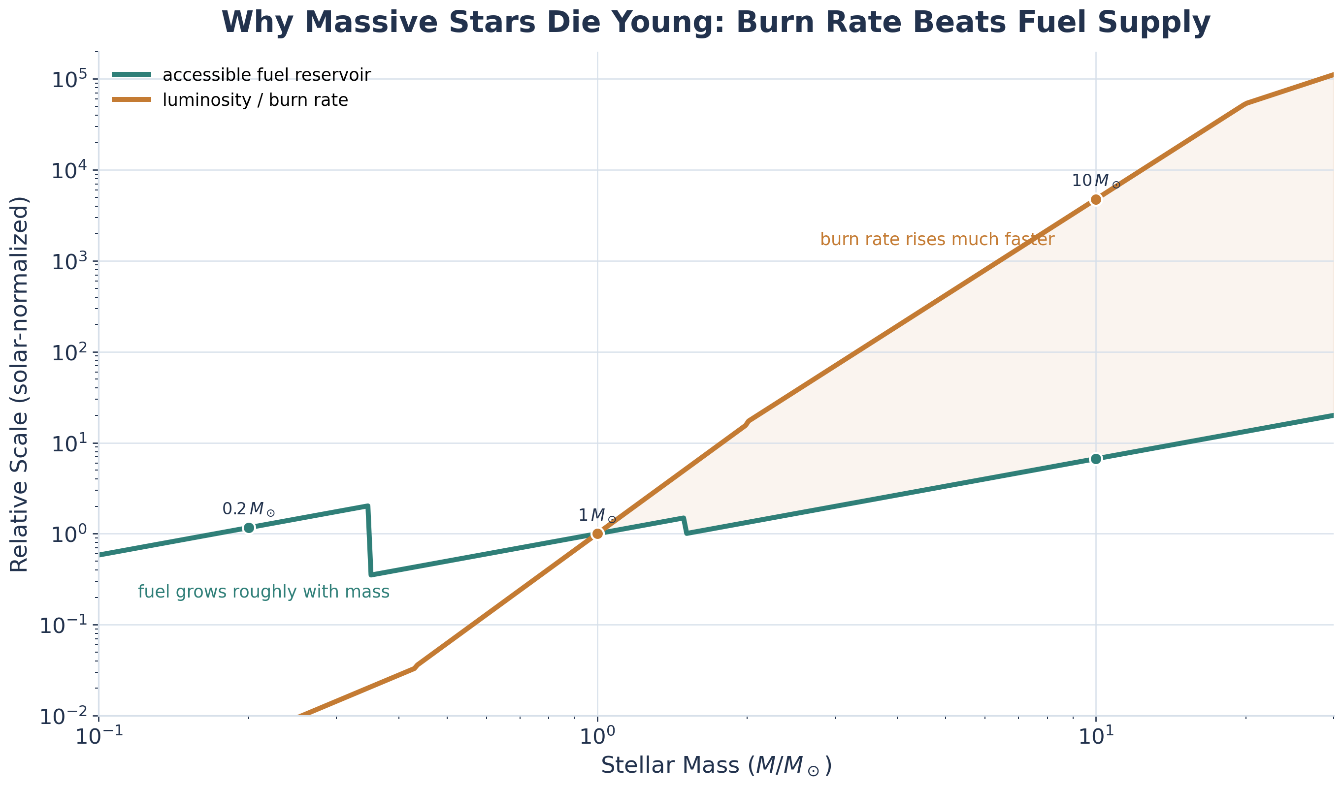
The accessible fuel supply rises with mass, but the luminosity rises much faster.
Why Normalize to the Sun?
Ratio method
- Write the star equation.
- Write the solar equation.
- Divide.
- Cancel shared units.
- Read the scaling.
Given: \(M = 2\,M_\odot\), \(L = 10\,L_\odot\)
Want: \(\dfrac{\tau_{\text{nuc}}}{\tau_{\text{nuc},\odot}}\)
Solar-Normalized Example: Show the Algebra
\[ \frac{\tau_{\text{nuc}}}{\tau_{\text{nuc},\odot}} \approx \left(\frac{2\,\cancel{M_\odot}}{1\,\cancel{M_\odot}}\right) \left(\frac{10\,\cancel{L_\odot}}{1\,\cancel{L_\odot}}\right)^{-1} \]
\[ = 2 \times 10^{-1} = 0.2 \]
This star gets only 20% of the Sun’s main-sequence lifetime.
Clock 1: Dynamical Response
\[ \tau_\text{dyn} \sim \frac{1}{\sqrt{G\bar{\rho}}} \tag{1}\]
- structural response clock
- set mainly by mean density
- not the age of the star
Mean Density Is the Compactness Shortcut
\[ \bar{\rho} = \frac{3M}{4\pi R^3} \]
smaller radius at fixed mass → larger density
larger density → shorter dynamical time
Solar-Normalized Dynamical Clock
\[ \frac{\tau_{\text{dyn}}}{\tau_{\text{dyn},\odot}} = \left(\frac{\bar{\rho}}{\bar{\rho}_\odot}\right)^{-1/2} = \left(\frac{M}{M_\odot}\right)^{-1/2} \left(\frac{R}{R_\odot}\right)^{3/2} \]
\(G\) cancels, so the ratio keeps only the physics that changes from star to star.
For the Sun, the Response Time Is Shockingly Short
\[ \tau_{\text{dyn},\odot} \approx 3 \times 10^3\,\text{s} \]
50 minutes
Structural imbalances get corrected very quickly.
Clock 2 Setup: The Gravitational Energy Reservoir
\[ E_{\text{grav}} \sim \frac{GM^2}{R} \]
More mass → deeper gravitational well
Larger radius → weaker binding
This is the energy gravity can release if the star contracts.
Luminosity Is the Energy Loss Rate
\[ L = \frac{\Delta E}{\Delta t} \]
Luminosity is power.
It tells us how fast the star is losing energy.
\[ \text{timescale} \sim \frac{\text{available energy}}{\text{energy loss rate}} \]
Clock 2: The Kelvin-Helmholtz Timescale
\[ \tau_\text{KH} \sim \frac{E_{\text{grav}}}{L} \]
\[ \tau_\text{KH} \sim \frac{GM^2}{RL} \]
Gravity-only lifetime = gravitational reservoir / luminosity.
For the Sun, Gravity Lasts Only
\[ \tau_{\text{KH},\odot} \approx 3 \times 10^7\,\text{yr} \]
30 million years
Gravity alone cannot power the Sun for billions of years.
Solar-Normalized Thermal Clock
\[ \frac{\tau_{\text{KH}}}{\tau_{\text{KH},\odot}} = \left(\frac{M}{M_\odot}\right)^2 \left(\frac{R}{R_\odot}\right)^{-1} \left(\frac{L}{L_\odot}\right)^{-1} \]
- more mass → more binding energy
- larger radius → weaker binding
- larger luminosity → faster spending
The Kelvin Problem
Kelvin’s model gave the Sun only tens of Myr.
Geology needed much more time.
Biology needed much more time.
The model was missing a deeper energy source.
Kelvin vs. the Geologists
Why Kelvin sounded reasonable
- careful energy bookkeeping
- gravity really does release energy
Why Kelvin failed
- the reservoir was too small
- fusion supplied the missing budget
Why \(E = mc^2\) Changes the Budget
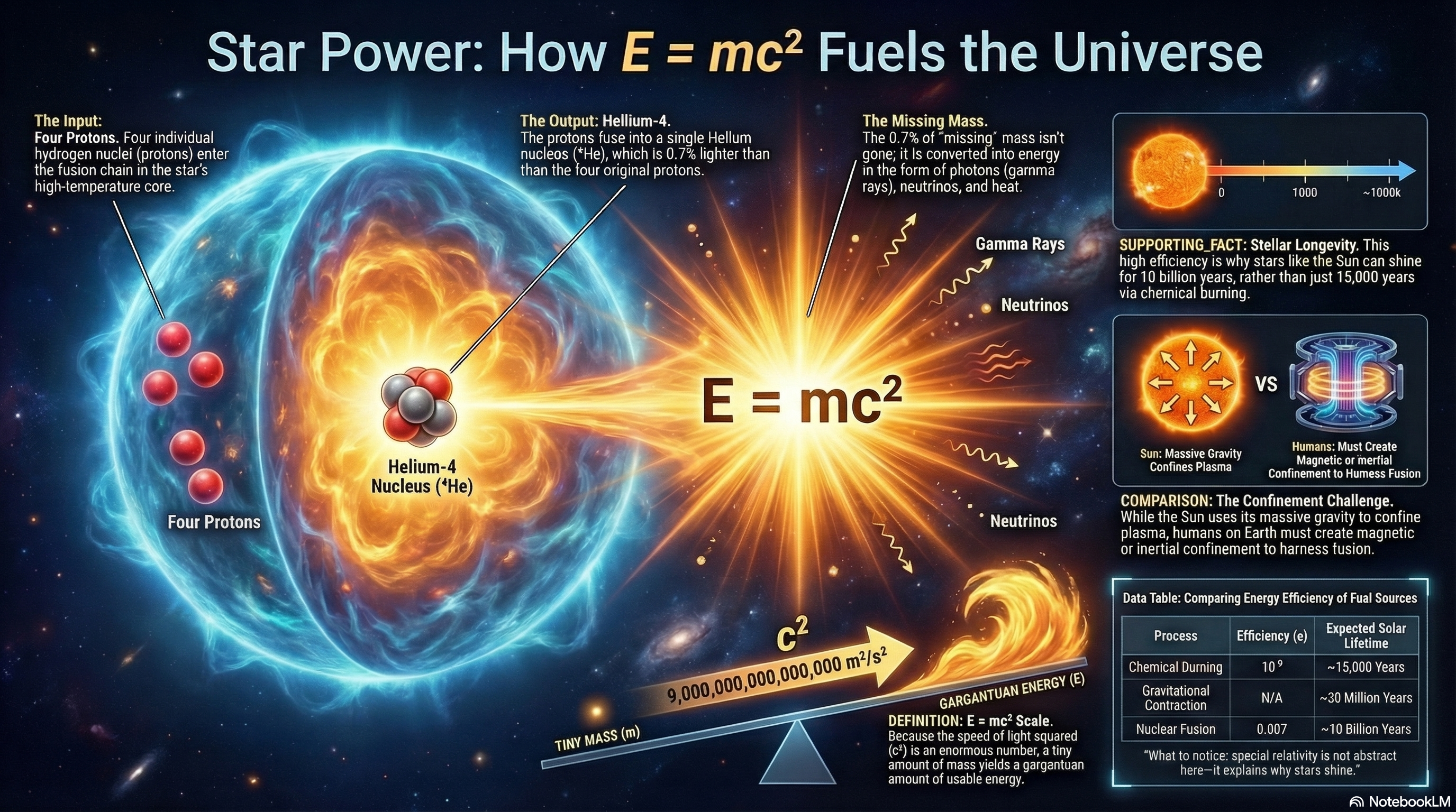
\[ \Delta E = \Delta m\,c^2 \]
Fusion taps rest-mass energy, not just thermal or chemical energy.
Clock 3: The True Main-Sequence Clock
\[ \tau_\text{nuc} \sim \frac{\varepsilon f_M M c^2}{L} \tag{2}\]
- \(\varepsilon\): fusion efficiency
- \(f_M\): accessible fuel fraction
- \(L\): burn rate
Now the Sun can last billions of years.
Full Normalized Nuclear Clock
\[ \begin{aligned} \frac{\tau_{\text{nuc}}}{\tau_{\text{nuc},\odot}} \approx\;& \left(\frac{\varepsilon}{\varepsilon_\odot}\right) \left(\frac{f_M}{f_{M,\odot}}\right) \left(\frac{M}{M_\odot}\right) \\ &\times \left(\frac{L}{L_\odot}\right)^{-1} \end{aligned} \]
\(\varepsilon\) is similar for H \(\rightarrow\) He fusion, but \(f_M\) can vary.
Solar-Normalized Nuclear Clock
\[ \frac{\tau_{\text{nuc}}}{\tau_{\text{nuc},\odot}} \approx \left(\frac{M}{M_\odot}\right) \left(\frac{L}{L_\odot}\right)^{-1} \]
Fuel in the numerator
Burn rate in the denominator
The core competition is still fuel / burn rate.
For the Sun, the Nuclear Clock Is
\[ \tau_{\text{nuc},\odot} \approx 10^{10}\,\text{yr} \]
10 billion years
That is why fusion solves Kelvin’s age problem.
Worked Example: A Fully Convective M Dwarf
Given: \(M = 0.2\,M_\odot\), \(L \approx 0.008\,L_\odot\)
Given: \(f_M \approx 10\,f_{M,\odot}\) for a fully convective star
Want: \(\dfrac{\tau_{\text{nuc}}}{\tau_{\text{nuc},\odot}}\)
Set up the ratios first so the algebra has somewhere to go.
M-Dwarf Lifetime: The Result
\[ \begin{aligned} \frac{\tau_{\text{nuc}}}{\tau_{\text{nuc},\odot}} &\approx \left(\frac{\cancel{\varepsilon}}{\cancel{\varepsilon_\odot}}\right) \left(\frac{10\,\cancel{f_{M,\odot}}}{1\,\cancel{f_{M,\odot}}}\right) \left(\frac{0.2\,\cancel{M_\odot}}{1\,\cancel{M_\odot}}\right) \left(\frac{0.008\,\cancel{L_\odot}}{1\,\cancel{L_\odot}}\right)^{-1} \\ &= 10 \times 0.2 \times \frac{1}{0.008} \approx 250 \end{aligned} \]
250 \(\tau_\odot\)
Low-mass stars can outlive the current universe by orders of magnitude.
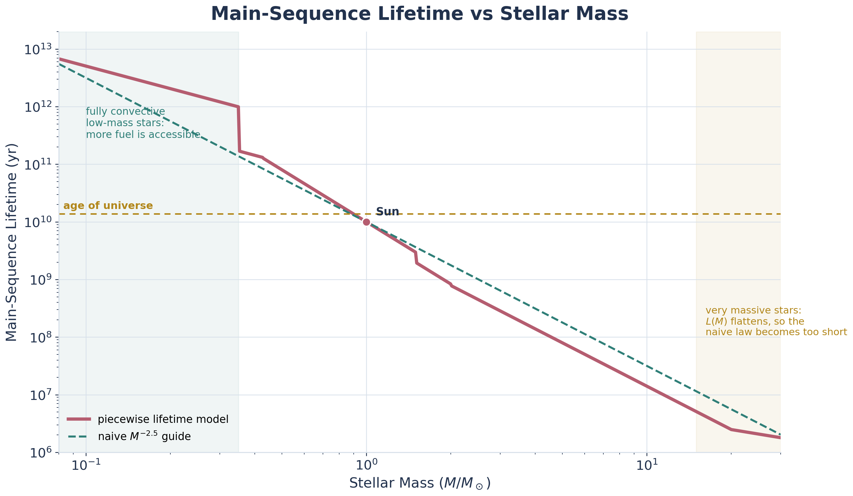
Fast Scaling Derivation
\[ \tau \sim \frac{\text{fuel}}{\text{burn rate}} \]
\[ \tau \sim \frac{M}{L} \]
\[ L \propto M^{3.5} \]
\[ \tau \propto M^{-2.5} \]
Why Massive Stars Die Young
\[ \frac{\tau_{\text{MS}}}{\tau_{\text{MS},\odot}} \approx \left(\frac{M}{M_\odot}\right)^{-2.5} \]
More mass → more fuel
More mass → MUCH higher luminosity
Extra fuel does not keep up.
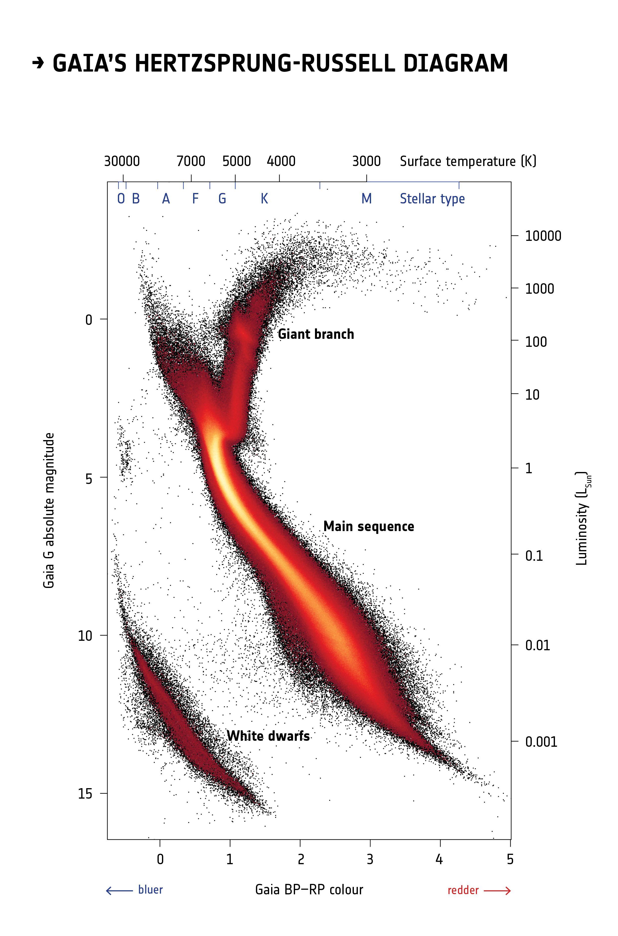
The Scaling That Explains the HR Diagram
How the Three Stellar Clocks Change with Mass
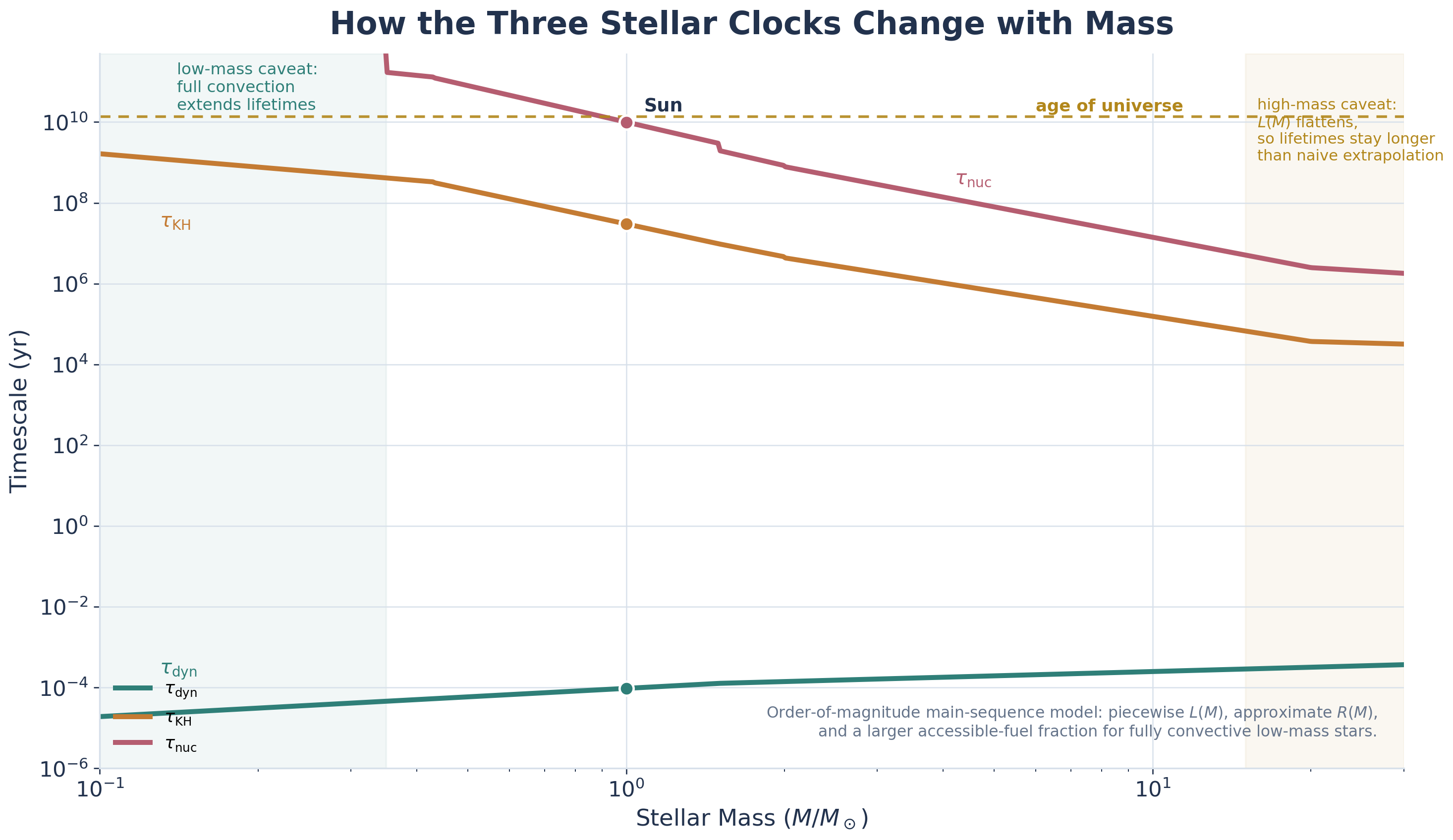
The hierarchy remains huge even as the thermal and nuclear clocks shrink for massive stars.
The Three Clocks, Side by Side
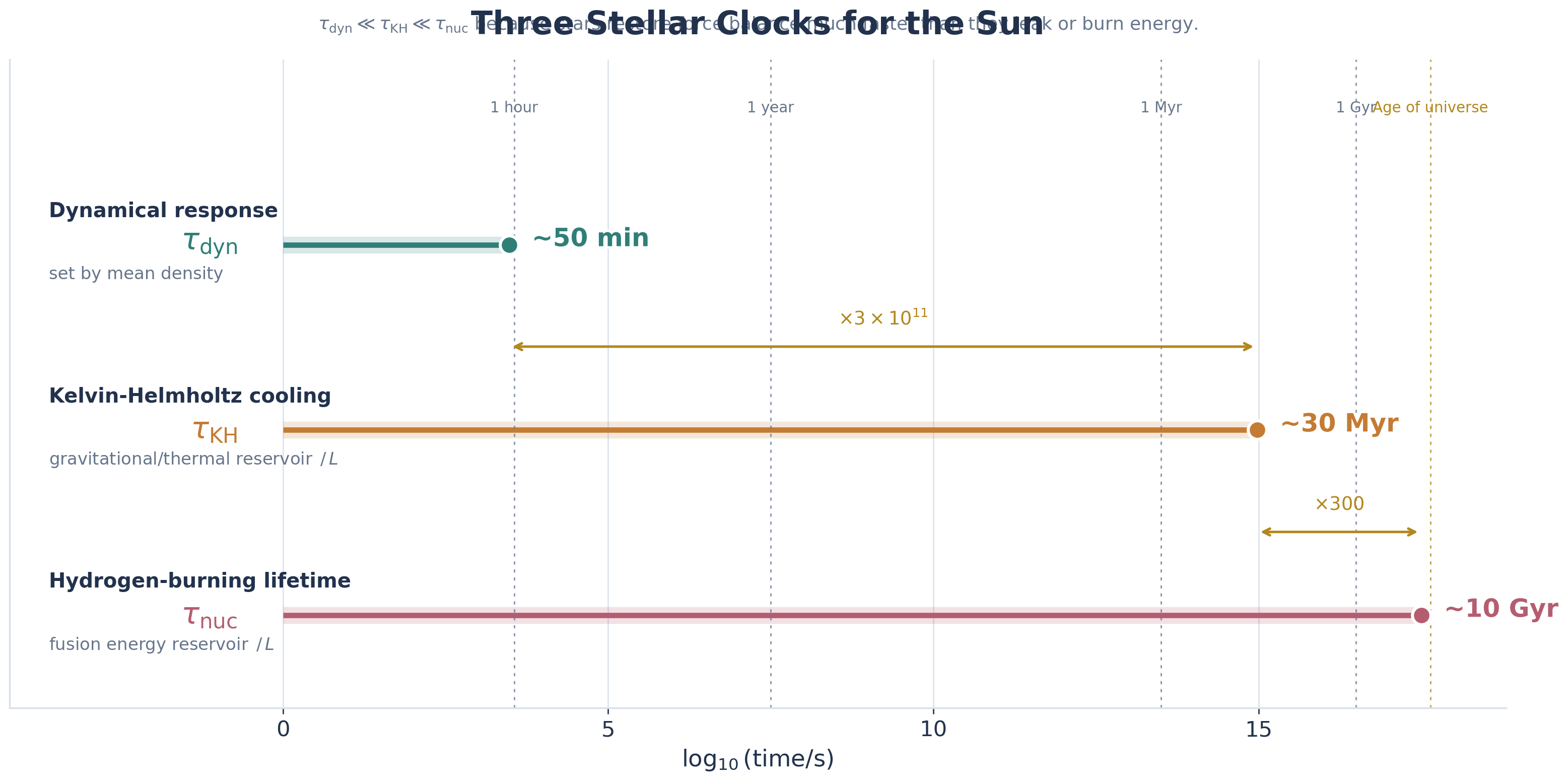
\[ \tau_{\text{dyn}} \ll \tau_{\text{KH}} \ll \tau_{\text{nuc}} \]
Turnoff Is an Age Clock
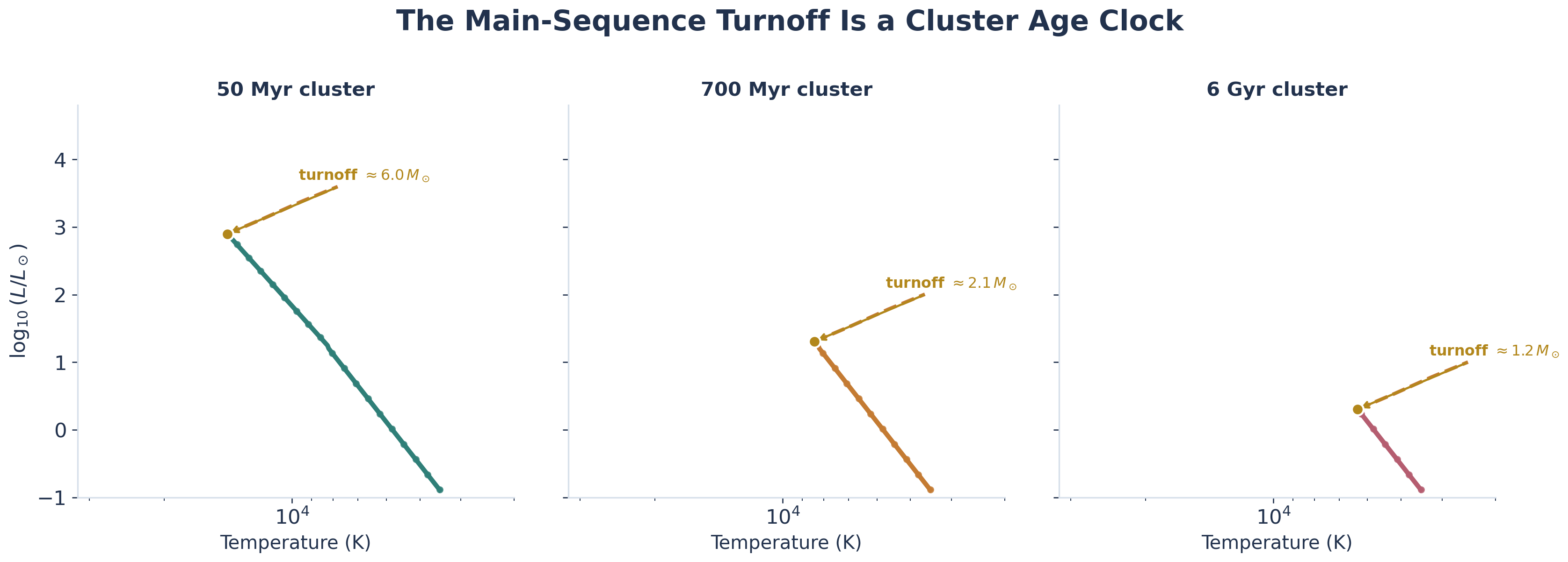
The most massive star still on the main sequence sets the cluster age.
Summary
- stars are clocks
- three timescales matter
- fusion sets the true lifetime
- turnoff turns the HR diagram into a timeline
Looking Ahead
If the Sun would collapse in about 50 minutes without support,
what is actually holding it up?
Next time: hydrostatic equilibrium