Part II: Gaussian Processes - Foundations and Theory
From Expensive Simulations to Fast Emulators | Module 6: The Learnable Universe | ASTR 596
“All models are wrong, but some are useful. The practical question is not whether to use a model, but which model to use.”
George E. P. Box
Learning Outcomes
By the end of Part II, you will be able to:
Articulate why surrogate modeling is essential for modern computational astrophysics and identify when emulation is appropriate
Explain Gaussian Processes as probability distributions over functions and derive predictions from Gaussian conditioning
Decide when to use GPs versus neural networks versus other approaches based on problem characteristics
Interpret kernel functions as encoding physical assumptions about smoothness, periodicity, and structure
Distinguish epistemic from aleatoric uncertainty and explain how GPs quantify both
Connect GP regression to the Bayesian inference framework from Module 5, seeing it as infinite-dimensional parameter inference
Apply GP concepts to emulate N-body star cluster simulations, predicting cluster evolution from initial conditions
The Big Picture: The Computational Crisis in Modern Astrophysics
The Problem We’re Solving
You’ve spent the semester building physics from first principles:
Module 1-2: Statistical Foundations
Central Limit Theorem, Maximum Entropy, moments as information compression
Statistical mechanics: from microstates to macrostates
The Boltzmann equation: evolution of distribution functions
Module 3: Dynamics in Phase Space
Collisionless Boltzmann equation for stellar systems
Virial theorem: when systems reach equilibrium
Two-body relaxation: how clusters dissolve
Module 4: Radiative Transfer
Photon transport through stellar atmospheres
Monte Carlo methods for solving integral equations
Importance sampling: making rare events tractable
Module 5: Bayesian Inference
Beliefs as probability distributions over parameters
MCMC (Markov Chain Monte Carlo): sampling complex posteriors when no closed form exists
Model comparison via marginal likelihoods
Projects 2, 3, 5: Building the Machinery
N-body simulations of star cluster evolution (gravity from scratch)
Monte Carlo radiative transfer (photon-by-photon tracking)
JAX implementations (fast, differentiable, GPU-accelerated)
JAX: Just-In-Time compiled array computing for Python with automatic differentiation
GPU: Graphics Processing Unit (massively parallel hardware accelerator)
JIT: Just-In-Time compilation (
jit) for speed
Each simulator encodes centuries of physics compressed into a few hundred lines of code. They work beautifully. They give correct answers.
They’re also prohibitively slow.
Output: Cluster properties at time , where the dynamical time is defined as (the characteristic timescale for orbital motion at the half-mass radius)
Note on Plummer profiles: For the Plummer density profile you’re using, the half-mass radius relates to the scale radius as (the exact factor depends on definitions and conventions; verify in your simulator’s documentation). So clusters with larger have longer dynamical times (slower evolution): . This means directly controls the evolutionary timescale—important for interpreting your emulator’s learned lengthscale !
Bound fraction: what percentage of stars remain gravitationally bound?
Core radius : how compact is the cluster center?
Half-mass radius : characteristic size
Velocity dispersion : kinetic energy indicator
Computational Cost:
Single simulation: ~10 minutes (1000 particles, 100 timesteps, direct N-body)
With your JAX implementation: ~2 minutes (GPU acceleration,
jitcompilation)
Now suppose you want to answer scientific questions:
Parameter Space Exploration: “Which initial conditions lead to cluster survival vs dissolution?”
Need: ~5,000 simulations to sample 3D space densely (roughly points per dimension for total)
Cost: 5,000 × 2 min = ~167 hours = 7 days of compute
Bayesian Parameter Inference: “What initial conditions produced the Pleiades cluster?”
Need: ~100,000 MCMC samples × likelihood evaluations
Cost: 100,000 × 2 min = ~3,333 hours = 138 days = 4.5 months
Optimization: “What initial setup maximizes cluster lifetime?”
Need: ~50,000 gradient evaluations for optimization
Cost: 50,000 × 2 min = ~1,666 hours = 69 days = 2.3 months
This is not a toy problem. This is real research.
### The Traditional Approach: Suffer or Approximate

Historically, astronomers faced a choice:

**Option 1: Just Wait**

- Run the expensive simulations
- Use supercomputers, parallelize, optimize
- Wait weeks/months for results
- **Problem**: Kills iteration speed, makes exploration impossible

**Option 2: Use Simple Models**

- Fit polynomials, power laws, linear regression
- Fast to evaluate, easy to interpret
- **Problem**: Physics is nonlinear, complex, high-dimensional. Simple models fail.

**Option 3: Dimensional Reduction**

- Derive simplified analytic approximations (e.g., virial theorem $Q = 1$ for equilibrium)
- Use scaling relations (e.g., $t_{\rm relax} \propto N / \ln N$)
- **Problem**: Valid only in limited regimes, miss interesting dynamics (unless validated with new simulations)

**Option 4: Give Up on Some Questions**

- Don't do parameter inference, don't optimize, don't explore broadly
- **Problem**: Science suffers

### The Modern Solution: Emulation

**Key Insight**: Your simulator $f_{\rm sim}$ is deterministic (or nearly so). Once you fix initial conditions $\mathbf{x}$, the output $y$ is determined by physics:

$$
y = f_{\rm sim}(\mathbf{x}) + \epsilon
$$

where $\epsilon$ represents numerical noise (finite timesteps, roundoff errors, stochastic elements).

**The Emulation Strategy**:

1. **One-Time Investment**: Run $N = 200\text{-}500$ simulations with carefully chosen initial conditions
   - Cost: $500 \times 2 \text{ min} \approx 16 \text{ hours}$ (one night of compute)
   - Generate training dataset: $\mathcal{D} = \{(\mathbf{x}_i, y_i)\}_{i=1}^N$

2. **Learn the Function**: Train a *surrogate model* (emulator) $f_{\rm emu}$ that approximates $f_{\rm sim}$
   - Cost: Minutes to hours (one-time training)
   - Result: Fast function $f_{\rm emu}(\mathbf{x})$ that mimics $f_{\rm sim}(\mathbf{x})$

3. **Deploy Everywhere**: Use $f_{\rm emu}$ instead of $f_{\rm sim}$ for:
   - Parameter space exploration: evaluate $f_{\rm emu}$ at millions of points
   - MCMC sampling: cheap likelihood evaluations
   - Optimization: fast gradient computation (if emulator is differentiable)
   - **Speedup**: $10^4$ to $10^6$ times faster than simulator

4. **Quantify Trust**: Emulator provides **uncertainty estimates**
   - "I predict bound fraction = $0.65 \pm 0.08$"
   - Know when to trust predictions, when to run more simulations
   - Principled decision-making about computational budget

:::{admonition} Connection to Module 5: Bayesian Inference
:class: note

In Project 4, you used MCMC to sample posterior distributions:

$$
p(\theta | \mathcal{D}) \propto p(\mathcal{D} | \theta) \, p(\theta)
$$

Each MCMC step required evaluating the likelihood $p(\mathcal{D} | \theta)$. When your model was simple (e.g., Gaussian with unknown mean/variance), this was cheap—just compute a probability.

But what if the likelihood requires *running a simulation*?

$$
p(\mathcal{D} | \theta) = p(\text{observed cluster properties} | \text{initial conditions } \theta)
$$

Then each MCMC step costs 2 minutes, and 100,000 samples = 138 days. **Intractable.**

**Emulation makes Bayesian inference feasible**: Replace $f_{\rm sim}(\theta)$ with $f_{\rm emu}(\theta)$ in the likelihood. Now each MCMC step costs milliseconds, and 100,000 samples = 1 hour.

This workflow is called **simulation-based inference** or **likelihood-free inference**, and it's how modern experiments (LIGO, DESI, Planck) constrain cosmological and astrophysical parameters.
[FIGURE 1.1: Emulation Workflow]
View Figure: Complete Emulation Workflow from Simulation to Inference
Figure 1.1: The complete emulation workflow. Red (expensive): Run your physics simulator 100-500 times at carefully chosen design points. Blue (training): Collect training dataset linking initial conditions to outcomes. Green (GP): Train Gaussian Process emulator that learns this mapping and provides uncertainty estimates μ(θ) ± σ(θ). Yellow (fast): Query emulator millions of times for parameter inference, sensitivity analysis, and exploration. The one-time upfront cost enables downstream analyses that would be impossible with the direct simulator.
Key Insight: GPs provide both prediction μ(θ) AND uncertainty σ(θ), enabling trustworthy predictions with error bars, adaptive sampling (add more training data where uncertain), and rigorous parameter inference (uncertainty propagation in MCMC).
First Principles: Why Gaussian Processes Work
The Core Idea: Functions as Infinite-Dimensional Vectors
You’re familiar with probability distributions over scalars and vectors:
Scalar random variable:
Describes uncertainty about a single number
Specified by mean and variance
Vector random variable:
Describes uncertainty about numbers jointly
Specified by mean vector and covariance matrix
A Gaussian Process extends this to functions:
Describes uncertainty about an entire function
Specified by:
Mean function (often after centering data)
Kernel function (covariance between function values)
Key Notation (Quick Reference)
| Symbol | Meaning | Type |
|---|---|---|
| Unknown function we’re learning | scalar | |
| Input (e.g., initial conditions ) | D-dimensional vector | |
| Output (e.g., bound fraction) | scalar | |
| Training dataset | pairs | |
| Design matrix () | matrix | |
| Training targets (vector of length ) | vector | |
| Gaussian process with mean and kernel | stochastic process | |
| Mean function | scalar function | |
| Kernel (covariance) function | scalar | |
| Kernel matrix () with entries | matrix | |
| Signal variance (prior amplitude) | scalar (output) | |
| Lengthscale (correlation distance) | scalar (input units) | |
| Noise variance (aleatoric uncertainty) | scalar (output) | |
| Hyperparameters | vector | |
| Predictive mean at test point | scalar | |
| Predictive epistemic variance at test point | scalar (output) |
Definition (Gaussian Process):
A stochastic process is a Gaussian Process if, for any finite collection of input points , the joint distribution of function values is a multivariate Gaussian:
Intuition:
A function is an infinite-dimensional object: it assigns a value to every point in input space
A GP says: “I don’t know the exact function, but I have beliefs about what it looks like”
Those beliefs are encoded in the kernel : “how similar should and be?”
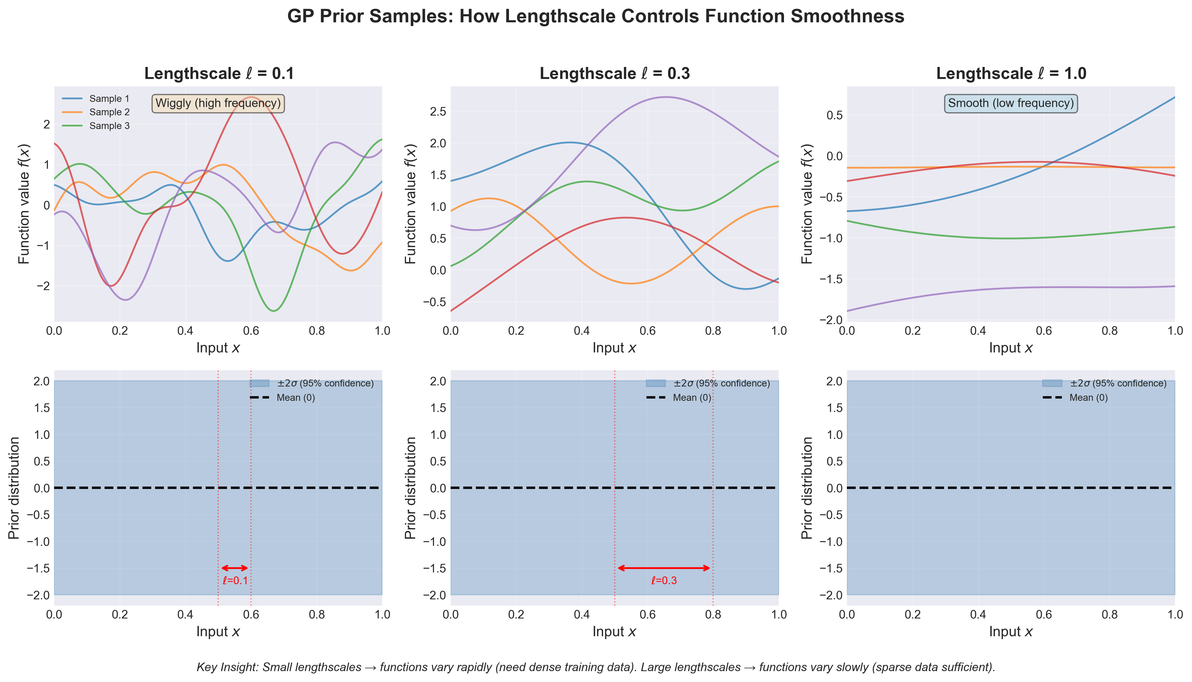
Figure 1:Figure 2.1: GP Prior Samples - How Lengthscale Controls Smoothness. Random function samples from GP(0, k_SE) with different lengthscales demonstrate how ℓ controls function smoothness. Top row: Individual samples show that small ℓ = 0.1 produces highly wiggly (high-frequency) functions, while large ℓ = 1.0 produces smooth (low-frequency) functions. Bottom row: Prior confidence bands (±2σ) with correlation length visualization. The red arrows show the lengthscale ℓ—the distance over which function values remain correlated (correlation drops to ~60% at distance ℓ). Key Insight: Small lengthscales require dense training data to capture rapid variations; large lengthscales allow sparse sampling since the function varies slowly.
From Finite to Infinite: The Consistency Requirement
Why use Gaussians for functions? Two reasons:
1. Computational Tractability
Gaussian distributions have magical properties (recall Module 1):
Marginals are Gaussian (if you ignore some dimensions, what’s left is still Gaussian)
Conditionals are Gaussian (if you observe some values, predictions for others are Gaussian)
Linear transformations are Gaussian
These properties mean we can compute predictions in closed form — no MCMC, no numerical integration, just linear algebra.
2. Consistency Under Marginalization
Suppose I specify a GP prior . Then by definition:
But also:
Consistency: The distribution over obtained by marginalizing out from the 3D Gaussian must match the 2D Gaussian. Gaussians satisfy this automatically.
This is called the Kolmogorov consistency theorem, and it’s why GPs are mathematically well-defined even though functions are infinite-dimensional.
🔴 The Mathematical Machinery: Gaussian Conditioning
Reviewing Multivariate Gaussians
Before we predict with GPs, we need the key formula from Module 1: Gaussian conditioning.
Suppose we have a joint Gaussian distribution over two sets of variables:
where:
are observed variables (training data)
are unobserved variables (test points)
(covariance is symmetric)
Question: If we observe (actual data), what is the distribution of ?
Theorem (Gaussian Conditioning):
The conditional distribution is Gaussian:
where:
This is the entire machinery of Gaussian Process regression.
Interpreting the Formulas
Let’s unpack these equations physically:
Posterior Mean
Prior guess: (what we’d predict before seeing data)
Residual: (how much the observations differ from prior expectations)
Regression weights: (how much each observation influences the prediction)
Update: Add weighted combination of residuals to prior
Physical interpretation: If test point is highly correlated with training point (large ), then observing strongly influences prediction at .
Posterior Covariance
Prior uncertainty: (uncertainty before seeing data)
Reduction: (how much observations reduce uncertainty)
Key insight: Posterior covariance does not depend on observed values !
Physical interpretation: Uncertainty depends only on where you observed data (the ), not on what you observed (the ). This makes sense: uncertainty is about information geometry, not values.
From Conditioning to GP Prediction
Now apply this to Gaussian Processes. We have:
Training data: where
Collected input-output pairs from expensive simulator
Noise (numerical errors, stochasticity)
GP prior:
Before seeing data, we believe has mean function and kernel
For simplicity, often take (data can be centered)
Goal: Predict at new test point
Setup: Form joint distribution over training outputs and test output:
where:
(training outputs, observed)
(test output, unobserved)
with (training-training covariance)
with (training-test covariance)
(test-test covariance, usually 1 for normalized kernels)
accounts for observation noise
Apply Gaussian conditioning: Condition on observed to get posterior over :
These are the fundamental equations of GP regression.
What These Equations Mean
Let’s interpret each term:
Predictive Mean:
Prior mean : Default guess (often zero)
Data term : How training outputs differ from prior expectations
Weights : How much influence each training point has (depends on noise and correlations)
Similarity : How similar test point is to each training point
Weighted average: Prediction is weighted sum of training residuals, weighted by similarity
Predictive Variance:
Prior variance : Uncertainty before seeing data (usually normalized to 1)
Reduction : How much training data reduces uncertainty
Key property: Variance is small (confident) when test point is similar to training points (large )
Another key property: Variance is large (uncertain) far from training data
Optional: Heteroskedastic Noise (Advanced)
So far we’ve assumed homoskedastic noise: is constant across all training points.
In reality, some simulators are noisier at certain parameter values:
Simulations of chaotic systems (butterfly effect) produce noise that scales with system sensitivity
Measurements in crowded stellar fields have position-dependent noise
N-body simulations may have higher variance for specific (Q, N, a) combinations
Heteroskedastic GP (input-dependent noise) uses :
When to use:
Variance clearly depends on inputs (inspect training residual scatter vs parameters)
You have repeated measurements at some points (allows fitting noise model)
Implementation: More complex; requires either:
Gaussian approximation + marginal likelihood optimization (GPyTorch, TensorFlow Probability handle this)
Approximate inference (EP, variational methods)
Pre-transform data to homoskedastize (log for multiplicative noise)
For your N-body emulation: Start with constant (homoskedastic). If residuals show structure (e.g., correlates with or ), ask instructors about heteroskedastic extensions.
🔴 Kernels: Encoding Physical Intuition
What Kernels Do
The kernel function is the heart of the GP. It encodes all your prior beliefs about the function you’re learning.
Definition: The kernel measures the covariance between function values at inputs and :
Interpretation:
Large → knowing tells you a lot about (strongly correlated)
Small → knowing tells you little about (weakly correlated)
→ prior variance of at any point (signal variance)
Key Properties (for a valid kernel):
Symmetry: (covariance is symmetric)
Positive Semi-Definite: For any set of points , the matrix must have non-negative eigenvalues
Stationarity (common but not required): Many kernels are stationary, (depends only on distance, not absolute location). Non-stationary kernels can model varying lengthscales (e.g., input warping, Gibbs kernel).
Why Positive Semi-Definite?
A covariance matrix must be positive semi-definite because:
for any vector . Variances can’t be negative!
Practical implication: You can’t just invent arbitrary . Must satisfy mathematical constraints. Common kernels (SE, Matérn, periodic) are guaranteed to be valid.
The Squared Exponential (RBF) Kernel
The most common kernel is the Squared Exponential (SE), also called Radial Basis Function (RBF):
Hyperparameters:
: Signal variance (overall amplitude of function, units: output)
: Lengthscale (how far you must move in input space for function to change significantly, units: input)
Anisotropic version (Automatic Relevance Determination - ARD):
When dimensions have different importance, use per-dimension lengthscales:
where each controls sensitivity to dimension . Small → high sensitivity, large → low sensitivity.
Physical interpretation:
Exponential decay: Correlation decreases exponentially with distance
Lengthscale: If , then (60% correlated)
Short lengthscale: Function varies rapidly, needs data points close together
Long lengthscale: Function varies slowly, data points far apart still informative
Infinite smoothness: Functions drawn from SE GP are infinitely differentiable (unrealistic for many physical systems!)
Visualization: Imagine bound fraction vs virial ratio :
Small : Bound fraction changes dramatically between and (highly sensitive)
Large : Bound fraction changes smoothly across entire range (insensitive)
The Matérn Family: More Realistic Smoothness
The SE kernel assumes infinitely smooth functions. Real physics is often rougher. The Matérn family allows tunable smoothness:
where:
: Smoothness parameter
: Modified Bessel function of the second kind
: Gamma function
Key cases:
(Matérn-1/2):
Equivalent to Ornstein-Uhlenbeck process
Functions are continuous but not differentiable (rough, can have kinks)
With :
Note: Still continuous! Doesn’t model true discontinuities, just permits roughness.
(Matérn-3/2):
Functions are once differentiable (smooth but can have kinks in second derivative)
With :
(Matérn-5/2):
Functions are twice differentiable (smoother, often good default)
With :
: Recovers SE kernel (infinitely smooth)
When to use which:
Matérn-5/2 (default): Start here for most physical systems (smooth but not unrealistically so)
Matérn-3/2: If Matérn-5/2 is over-smooth (under-coverage in calibration, residuals show structure)
SE: When you know function is truly smooth (interpolating well-behaved data)
Matérn-1/2: When function is rough/non-smooth, but still continuous (not for true discontinuities - GPs struggle with those)
Practical tuning guide:
If predictions are under-covered (empirical coverage < 68% at 1σ) → try lower (Matérn-3/2 instead of 5/2) or regularize
If predictions are numerically wiggly → increase (higher smoothness)
If lengthscales blow up → kernel may be too flexible, try Matérn-5/2 or SE
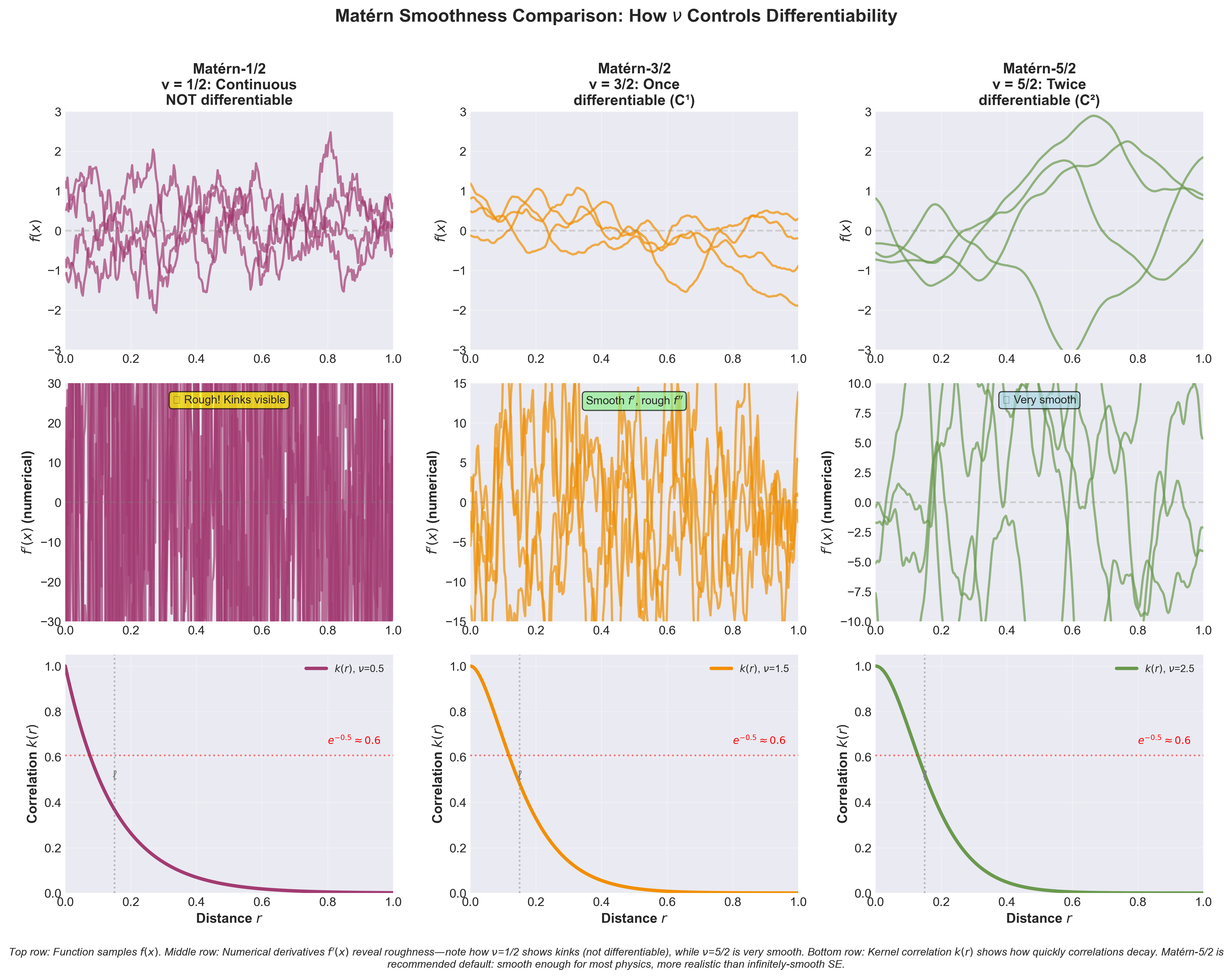
Figure 4:Figure 2.3: Matérn Smoothness Comparison. Matérn family smoothness comparison showing how ν controls differentiability. Top row: Function samples f(x) for each smoothness parameter. Middle row: Numerical derivatives f’(x) reveal roughness—Matérn-1/2 (ν=0.5) shows visible kinks and is NOT differentiable (rough, discontinuous slopes); Matérn-3/2 (ν=1.5) has smooth first derivatives but rough second derivatives (once differentiable); Matérn-5/2 (ν=2.5) is very smooth (twice differentiable). Bottom row: Kernel correlation k(r) vs distance shows how quickly correlations decay. Practical Recommendation: Use Matérn-5/2 as default for physics emulation—smooth enough for realistic systems but more flexible than infinitely-smooth SE kernel. Only use SE when you KNOW the function is truly infinitely smooth (rare in real physics). Use Matérn-3/2 if validation shows underfitting or if you expect rougher behavior.
Periodic Kernels: Exploiting Symmetries
If your function has periodic structure, you can encode this:
Note: This is the 1D periodic kernel. For vector inputs, periodicity is typically applied per dimension: . Use only if you have strong physical reason to expect periodicity in a specific dimension (e.g., orbital angular position, stellar rotation phase).
where:
: Period (units: input)
: Lengthscale within period (controls smoothness)
When to use:
Time series with known periodicity (stellar rotation, orbital period)
Spatial data with translational symmetry
N-body example: If you’re emulating cluster properties in a rotating frame, periodic kernel might capture rotational symmetry. (Rare, but possible!)
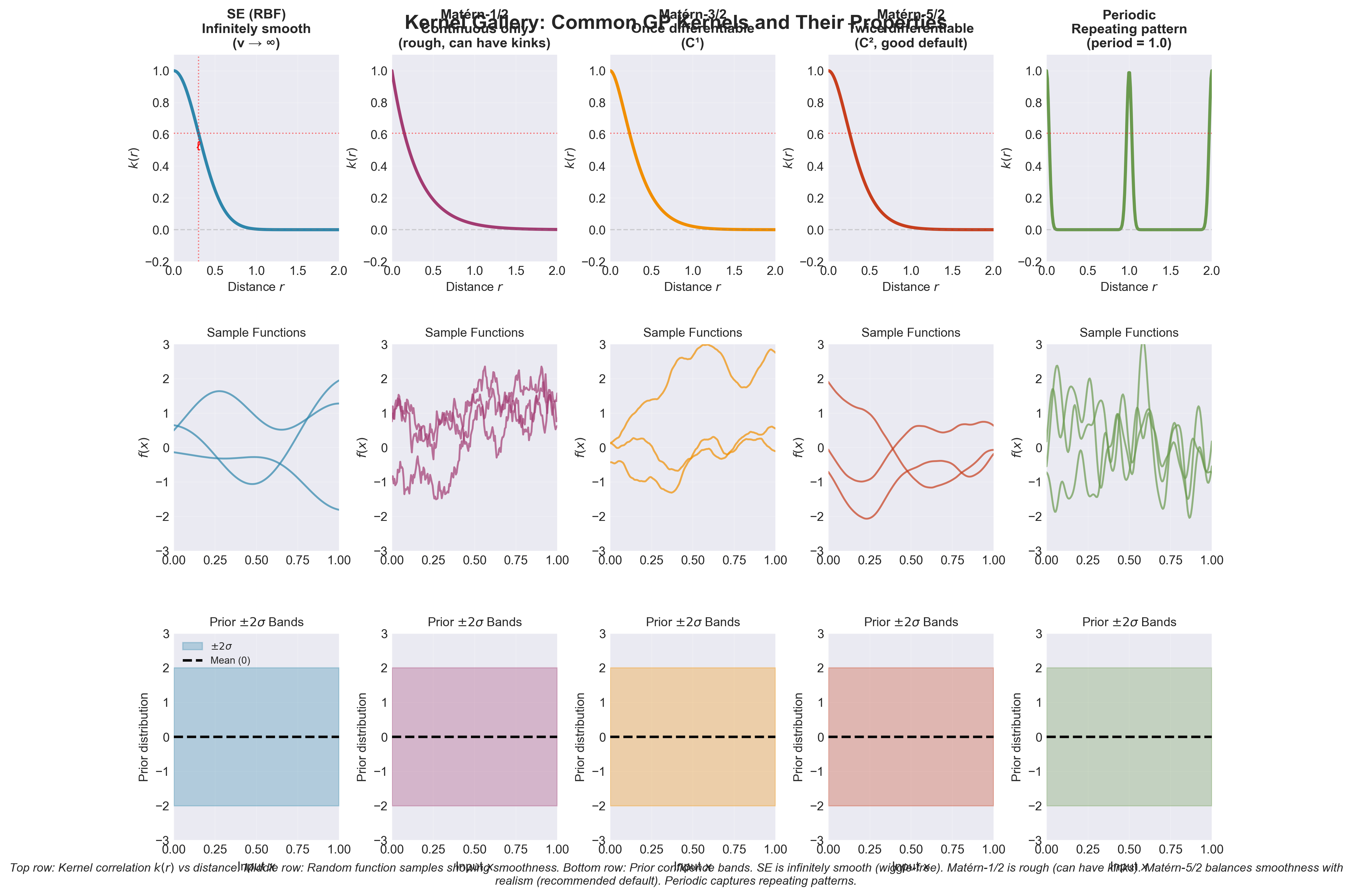
Figure 5:Figure 2.2: Kernel Gallery. Comprehensive kernel gallery comparing five common GP kernels. Top row: Kernel correlation k(r) vs distance r—shows how correlation decays with separation. SE (RBF) has smooth Gaussian decay; Matérn-1/2 has exponential decay (roughest); Matérn-3/2 and 5/2 are intermediate; Periodic shows repeating pattern. Middle row: Random function samples demonstrate smoothness—SE is infinitely smooth (no kinks ever), Matérn-1/2 can have kinks (rough), Matérn-5/2 is very smooth but more realistic than SE, Periodic captures repeating patterns. Bottom row: Prior ±2σ confidence bands show expected function variability. Key Comparisons: SE (blue) is too smooth for most physics; Matérn-1/2 (purple) is too rough (kinks visible); Matérn-5/2 (red) balances smoothness with realism (recommended default); Periodic (green) for phenomena with known periodicity. All kernels share lengthscale ℓ=0.3 for fair comparison.
Compositional Kernels: Building Complexity
You can combine kernels to build more complex priors:
1. Addition
Functions are sums of two independent processes
Example: Smooth trend + noise, Long-range + short-range structure
2. Multiplication
Functions have coupled structure
Example: Periodic function with varying amplitude
3. Per-dimension kernels:
Different structure in each dimension
Encodes independence assumptions
🔴 Decision Framework: When to Use What
You now understand what GPs are and how they work. But when should you actually use them?
The Method Landscape
Modern surrogate modeling has three main approaches:
| Method | Strengths | Weaknesses | When to Use |
|---|---|---|---|
| Polynomial / Basis Function Expansion | Simple, interpretable, fast | Limited flexibility, high-D curse | Linear systems, low-D, known structure |
| Gaussian Processes | Uncertainty quantification, data-efficient, interpretable hyperparameters | scaling, assumes smoothness, struggles in high-D | Low-D (-20), need uncertainty, limited data (), interpretability important |
| Neural Networks | Scales to high-D, handles complex patterns, can learn representations | Needs lots of data, uncertain uncertainty, black box | High-D (), abundant data (), complex discontinuities |
When to Use Gaussian Processes
GPs Excel When:
✅ Low-dimensional inputs (single-digit to low-tens, roughly –20)
Kernel methods scale poorly with dimension (curse of dimensionality)
Need exponentially more data to cover space as increases
Effective dimensionality often lower than nominal when using ARD (automatic relevance determination learns which dimensions matter)
Your N-body emulation: → perfect for GPs!
✅ Limited training data (-5000)
GPs are data-efficient (Bayesian priors help)
Can make reasonable predictions from tens of samples
NNs need thousands to millions of samples
✅ Uncertainty quantification is critical
GPs give Bayesian uncertainty automatically
Know when predictions are trustworthy
Essential for scientific applications (error bars matter!)
✅ Smooth or structured functions
Physics is usually continuous, differentiable
Kernels encode this structure explicitly
GPs exploit smoothness for efficient learning
✅ Interpretability matters
Hyperparameters have clear physical meaning
→ “Bound fraction changes significantly over ”
→ “Typical variation in bound fraction is ”
Can diagnose what GP learned about physics
✅ Need gradients
GP predictions are differentiable (can compute )
Useful for optimization, sensitivity analysis
JAX makes this automatic!
When NOT to Use Gaussian Processes
❌ High-dimensional inputs ()
Kernel evaluations become expensive
Need impractical amounts of data to cover space
Consider dimensionality reduction first, or use NNs
❌ Large datasets (-10,000)
training cost becomes prohibitive
memory for covariance matrix
Solution: Sparse/inducing-point GPs (see below)
Scaling Beyond : Sparse GPs
If you have abundant data () but still want GP uncertainty quantification, use sparse approximations:
Idea: Approximate full GP with inducing points:
Select representative locations in input space
Complexity: instead of
Memory: instead of
Methods:
Variational Free Energy (VFE) / Titsias (2009): Optimal inducing locations
SVGP: Stochastic variational GPs for
When to use:
You have simulations
Still want principled uncertainty (not just NN)
Willing to accept approximation error
Trade-off: Lose some accuracy for computational feasibility.
For your project: With , use exact GP. If extending to , consider sparse methods.
JAX Libraries: GPJax supports sparse GPs natively.
❌ Discontinuous or highly irregular functions
GPs assume some smoothness
Can’t represent sharp discontinuities well
Matérn-1/2 helps, but NNs might be better
❌ Complex structured outputs
GPs naturally handle scalar outputs
Multi-output GPs possible for moderate cases:
Independent GPs: Train separate GP per output (simple, loses correlations between outputs)
Multi-output GP (coregionalization): Model output correlations via cross-covariance (ICM/LMC methods)
Example: If and are correlated, joint GP can leverage this
Benefit: More data-efficient than training separate GPs if outputs are correlated
Caveat: More hyperparameters to optimize (cross-covariances + per-output lengthscales)
Trade-off: More complex training, but can improve predictions when training data is scarce
Your project: For , independent GPs are recommended (3× training cost, straightforward implementation, maintains modularity). Use multi-output only if data-scarce and outputs strongly correlated.
For high-dimensional outputs (images, sequences, graphs) → use NNs
❌ Real-time constraints
Training is one-time cost (acceptable if slow)
But prediction scales as for test points
If need millisecond inference for millions of queries, NNs may be faster
Decision Tree for Your N-Body Emulation
Let’s apply this to your project:
Your Problem:
Input: as primary parameters
is derived: (fixed IMF, M)
Output: Bound fraction, , etc. (scalar properties)
Training data: ~250 simulations (200 provided + 50 yours)
Goal: Predict at new initial conditions, quantify uncertainty
Analysis:
✅ → Low-dimensional (GPs shine here)
✅ → Limited data (GPs data-efficient)
✅ Smooth physics (cluster properties vary continuously with ICs)
✅ Need uncertainty (must know when emulator is trustworthy)
✅ Interpretability (want to understand which parameters matter)
Verdict: Gaussian Processes are ideal for this problem!
But also try Neural Networks because:
Good learning exercise (compare approaches)
NNs scale better if you want to add more simulations later
Can handle multi-output prediction more naturally
Shows you the tradeoffs empirically
[FIGURE 5.1: Emulation Method Decision Tree]
View Figure: Complete Decision Tree for Choosing Emulation Methods
Figure 5.1: Decision tree for choosing emulation methods based on problem characteristics. Green boxes: Recommended methods with strong theoretical/empirical support. Yellow boxes: Alternative methods to consider. Red boxes: Warning situations requiring problem reformulation. Blue diamonds: Decision points based on dimensionality, data availability, and smoothness assumptions. For your N-body cluster emulation (d=3, n≈250, smooth physics, need UQ), follow the path: d≤5 → Yes UQ → n<1000 → Standard GP with SE or Matérn kernel—the ideal choice!
Quick Reference: Standard GP (d≤5, n<1000) for small data + uncertainty. GP with ARD (5<d≤20) for automatic feature selection. Sparse GP (n>5000) for computational efficiency. Neural Networks (d>20 or n>10,000) for high-dimensional/large-data regimes. Decision Rule: Use GPs when you need rigorous uncertainty quantification, have limited expensive training data, smooth outputs, and interpretable lengthscales matter.
🎓 What We’ve Learned: Theory Summary
Let’s step back and see what we’ve covered in Part I.
First Principles
The Problem: Scientific simulations encode physics but are too slow for exploration, optimization, inference
The Solution: Emulation—learn a fast surrogate from modest training data
Why GPs Work:
Bayesian inference in function space
Gaussian conditioning gives predictions in closed form
Kernels encode physical structure (smoothness, lengthscales)
Uncertainty quantification is built-in (know when to trust predictions)
When to Use GPs:
Low-dimensional problems ()
Limited data ()
Smooth physics
Uncertainty matters
Interpretability desired
Connection to Everything You’ve Learned
Module 1 (Statistics):
GPs extend multivariate Gaussians to infinite dimensions
Central Limit Theorem: Why Gaussian assumptions are reasonable
Moments: GP mean and covariance are first two moments
Module 2-3 (Stellar Systems):
N-body simulations define functions
Emulation lets you explore phase space without full dynamics
Lengthscales relate to characteristic scales (dynamical time, relaxation time)
Module 4 (Radiative Transfer):
Monte Carlo RT is expensive (like N-body)
Could emulate emergent spectrum vs stellar parameters
Same workflow applies!
Module 5 (Bayesian Inference):
GPs are Bayesian: Prior (kernel) + Likelihood (data) = Posterior (predictions)
MCMC becomes tractable with emulator replacing expensive likelihood
Marginal likelihood for hyperparameters = evidence for model selection
Project 5 (JAX):
Automatic differentiation gives gradients for optimization
JIT compilation makes GP fast
Vectorization (
vmap) enables efficient prediction at many test pointsGPU acceleration makes feasible
The Philosophical Point
Machine learning is not magic. It’s principled probabilistic inference with mathematical foundations.
GPs exemplify this:
Every component has clear interpretation (kernel, hyperparameters, predictions, uncertainty)
Connections to statistics, physics, computation
Uncertainty quantification is first-class citizen (not afterthought)
Hyperparameters have physical meaning (not just numbers to tune)
When you implement a GP, you’re not using a black box—you’re applying a century of mathematics (Kolmogorov, Wiener, Rasmussen) to solve a 21st-century astrophysics problem.
This is computational astrophysics in 2025!
🔮 Preview: Part II
In Part II: GP Implementation, you’ll learn:
The complete emulation workflow (training data → predictions)
Hyperparameter optimization via marginal likelihood
Numerical implementation in JAX
Validation and diagnostics
How to use emulators for scientific inference
See you in Part II! Continue to Part II: Gaussian Processes - Implementation and Practice.
Self-Check Rubric: Do You Understand GPs?
Before Part II, honestly assess yourself using this rubric. This will help you identify gaps and ensure you’re ready for implementation.
1. Conceptual Understanding
Can you explain why Gaussians are special? (closure under conditioning and marginalization)
Can you explain what a kernel does in one sentence without using the word “covariance”?
Can you sketch how varies with position when you have training data at ?
Can you distinguish epistemic from aleatoric uncertainty and give an astrophysics example of each?
If you checked <3 boxes: Reread “First Principles” and “Uncertainty” sections before Part II.
2. Practical Knowledge
Can you list 5 hyperparameters of an SE kernel with ARD and explain what each controls?
Can you write pseudocode for computing from scratch? (triple loop is fine)
Can you explain why you should never compute explicitly?
Can you design a training dataset for emulating your N-body simulator? (what range of ? how many points?)
If you checked <3 boxes: Work through the “Kernels” and “Computational” sections with paper and pen.
3. Physical Intuition
Can you guess approximate lengthscales for each parameter in your star cluster problem?
Can you explain why extrapolating a GP beyond the training range is risky?
Can you sketch for a 1D problem with 3 training points?
Can you explain the connection between GP lengthscale and physical smoothness of your simulator?
If you checked <3 boxes: Reread the “Why This Matters” sections and think about your N-body simulations.
4. Implementation Readiness
Can you write a JAX function that computes the SE kernel for two input vectors?
Can you explain how to standardize training data and denormalize predictions?
Can you list 3 potential numerical stability issues and how to fix each?
Do you know what “jitter” is and approximately how large to make it?
If you checked <3 boxes: Start Part II prepared to learn; ask questions early.
Scoring:
14+ / 16 boxes checked: Ready for Part II! You have a solid conceptual foundation.
12-14: You’re close; review weak areas before starting Part II.
< 12: You’ll learn in Part II, but prioritize catching up on foundational concepts.
Note: Honest self-assessment helps you learn faster. If you’re uncertain about a box, leave it unchecked and revisit that topic.
📖 Glossary of Key Terms
ARD (Automatic Relevance Determination): Kernel with per-dimension lengthscales , allowing the GP to learn which input dimensions matter most. Small → high sensitivity to dimension , large → low sensitivity (GP effectively ignores that dimension).
LHS (Latin Hypercube Sampling): Stratified sampling method ensuring uniform coverage in each dimension separately. Better than random sampling for space-filling experimental designs. Widely used for training surrogate models.
OOD (Out-of-Distribution): Test points far from training data, where the emulator extrapolates and uncertainty is high. Detect via kernel similarity: (e.g., 0.05; validate empirically for your problem as threshold depends on learned hyperparameters).
ICM/LMC (Intrinsic Coregionalization Model / Linear Model of Coregionalization): Multi-output GP methods that model correlations between outputs via cross-covariance functions. Beyond scope of this course; see Álvarez et al. (2012) for details.
Epistemic Uncertainty: Uncertainty about the latent function (reducible with more training data). From GP: . Also called “model uncertainty” or “knowledge uncertainty.”
Aleatoric Uncertainty: Irreducible noise in observations (measurement error, simulation stochasticity). From likelihood: . Also called “data uncertainty.”
Marginal Likelihood (Evidence): , the probability of observing training data given hyperparameters, integrating over all possible functions. Used for Type-II maximum likelihood hyperparameter optimization. Implements Occam’s razor automatically.
Kernel (Covariance Function): , measures correlation between function values at inputs and . Encodes smoothness assumptions and prior beliefs about function structure.
Lengthscale (): Characteristic distance in input space over which function values remain correlated. Small → rapid variation (wiggly functions), large → smooth variation (slowly varying functions). Units: same as input dimensions.
Signal Variance (): Prior variance of function values (overall amplitude of variation). Units: output.
Noise Variance (): Observation noise level (aleatoric uncertainty). Units: output.
Cholesky Factorization: Decomposition where is lower-triangular. Numerically stable way to solve linear systems and compute determinants. Essential for GP implementation.
Jitter: Small constant added to kernel matrix diagonal to ensure numerical stability: . Prevents Cholesky failures from near-singular matrices. Typical values: (scale-aware).
SE (Squared Exponential) Kernel: Also called RBF (Radial Basis Function). Assumes infinitely smooth functions. Often too smooth for real physics.
Matérn Kernel: Family of kernels with tunable smoothness . Matérn-5/2 is recommended default (twice differentiable, realistic for physics).
PSD (Positive Semi-Definite): Property required for valid kernels. Ensures covariance matrices have non-negative eigenvalues (variances can’t be negative).
MCMC (Markov Chain Monte Carlo): Sampling method for complex posterior distributions (from Module 5). GPs enable MCMC-based inference by providing fast, differentiable emulators of expensive simulators.
JAX: Just-In-Time compiled array computing library for Python with automatic differentiation. Makes GP implementation fast and enables gradient-based hyperparameter optimization.
JIT (Just-In-Time Compilation): Compilation technique that speeds up Python code to near-C performance. Use @jit decorator in JAX.
vmap (Vectorized Map): JAX function for automatic vectorization. Maps a function over batch dimension efficiently (avoids Python loops).
Continue to Part II for implementation! 🚀
“The best way to understand a Gaussian Process is to implement one.” — Every computational scientist ever