Part 1: The Fundamental Paradox - Calculus on Computers
Foundations of Discrete Computing | Numerical Methods Module 1 | ASTR 596
Learning Outcomes
By the end of this section, you will be able to:
Explain why computers cannot take the limit and analyze the implications for numerical derivatives
Derive all finite difference approximations (forward, backward, central, higher-order) from Taylor series
Calculate the optimal step size by analyzing the trade-off between truncation error () and round-off error ()
Implement and evaluate all finite difference approximations with appropriate error handling
Predict error scaling behavior before running code and verify predictions empirically
Introduction: Why Numerical Derivatives Matter
Before diving into technical details, let’s understand why numerical derivatives and finite precision arithmetic are foundational to computational astrophysics. Nearly every calculation you’ll perform depends on these concepts.
Derivatives are everywhere in astrophysics:
Velocities and accelerations: Every N-body simulation computes
where is position, is velocity, and is acceleration.
Stellar structure: The equations of stellar evolution involve gradients like
where pressure, temperature, is the enclosed mass within radius
Radiative transfer: The change in intensity along a ray:
where is the path length traveled, is the opacity, and is the emissivity.
Orbital mechanics: Kepler’s equation for planetary motion requires finding where is eccentric anomaly.
Cosmological evolution: The Friedmann equations involve where is the scale factor of the universe.
Why numerical methods are essential: Most astrophysical problems cannot be solved analytically. Consider the three-body problem - there’s no closed-form solution for the general case. Instead, we must use numerical approximations, which means:
Converting continuous differential equations to discrete difference equations
Managing errors that arise from finite precision arithmetic
Balancing accuracy against computational cost
Understanding when our approximations break down
The computational challenge: In practice, astrophysical simulations must handle enormous dynamic ranges that push the limits of finite precision arithmetic:
Gravitational dynamics: N-body simulations track forces varying by factors up to ~1018 (from close binaries at ~0.01 AU to globular cluster scales at ~100 pc), exceeding the ~1016 dynamic range of double precision and forcing us to use hierarchical methods or separate coordinate systems
Star formation: Simulating giant molecular clouds requires resolving both the ~100 pc cloud scale and ~100 AU protostellar disks - a factor of 106 in length scale and 1011 in density (from 10-24 g/cm³ in the diffuse ISM to 10-13 g/cm³ in dense molecular cores)
Temporal evolution: Stellar evolution codes span from dynamical timescales (hours) to main sequence lifetimes (billions of years) - a factor of 1013 where errors accumulate at every timestep
Mixed scales: Galaxy simulations must resolve both individual star-forming regions (~1 pc) and galactic halos (~100 kpc), while maintaining energy and momentum conservation
Double precision provides only ~16 decimal digits. We cannot simultaneously represent these extreme scales with full precision. We must understand:
How computers represent numbers and where precision is lost
How errors propagate through calculations
How to reformulate problems for numerical stability
When to trust our results and when to be skeptical
This section provides the rigorous foundation you need to write reliable code for astrophysical simulations. The principles you learn here will apply to every project in this course and throughout your research career.
The Core Problem
Recall that the mathematical definition of a derivative of a function at a point is:
where represents a small displacement from the point . This definition relies on taking the limit as approaches zero - we evaluate the slope of secant lines through points that get arbitrarily close together until we obtain the slope of the tangent line at . The derivative is fundamental to physics, describing velocities, accelerations, and all forms of change.
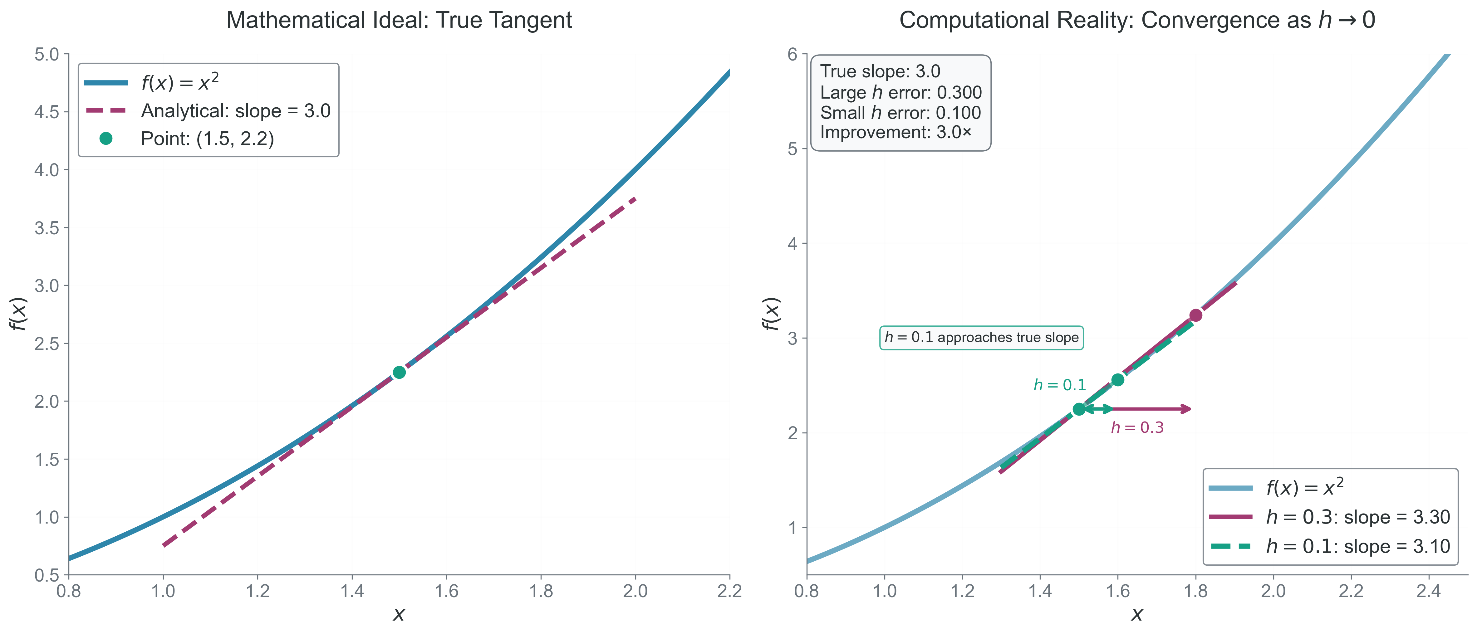
Figure 1:The derivative paradox: mathematical definition requires , but computers cannot take true limits. Left: analytical derivative (smooth tangent line). Right: numerical approximation using finite values showing convergence - smaller approaches the true slope better than larger .
On a computer, this mathematical ideal encounters a fundamental obstacle. Computers represent numbers using floating-point arithmetic with finite precision (typically 64 bits for a double-precision number).
This floating-point arithmetic means:
We cannot represent exactly - Division by zero would cause the program to crash or return undefined/infinite values.
We cannot make arbitrarily small - Below a certain threshold (around 10-16 for double precision), the computer cannot distinguish between and due to rounding. When we try to compute , both values round to the same floating-point number, giving us , which is completely wrong.
Even moderate values of cause problems - When is very small (say 10-10), and , we’re subtracting two nearly equal numbers. Due to finite precision, we might only retain a few significant digits in the difference, leading to catastrophic cancellation.
This catastrophic cancellation is one of the most common sources of numerical error in scientific computing.
Therefore, we must approximate the derivative using a finite difference:
This finite difference approximation creates a fundamental trade-off:
If is too large: The approximation is poor because we’re measuring the slope of a secant line far from the point of interest. This introduces truncation error proportional to .
If is too small: Floating-point round-off errors dominate. When and are nearly equal, their difference loses significant digits, and dividing by a tiny amplifies this error.
The optimal value of must balance these competing effects. Through rigorous analysis (which we’ll derive shortly), this optimal value turns out to be approximately for forward differences, where is the machine epsilon for double precision.
This machine epsilon represents the fundamental limit of floating-point precision. This fundamental limitation means that on a computer, we can typically only compute derivatives to about 8 digits of accuracy using forward differences, even though our numbers have 16 digits of precision. This is why understanding numerical methods is crucial.
The Complete Finite Difference Landscape
Now that we understand the fundamental challenge, let’s explore all the ways we can approximate derivatives numerically. Each method emerges from different manipulations of Taylor series, and each has distinct advantages and trade-offs.
Intuition: Why Taylor Series?
Taylor series answers the question: “How does a function change near a point?” It builds the function from its derivatives, like constructing a curve from its slope, curvature, and higher-order bending.
The Taylor series expansion of a function around a point is:
Or more compactly:
Each term adds more detail: the first gives the value, the second adds the slope, the third adds curvature, and so on. For numerical methods, we truncate this infinite series after a few terms, which introduces truncation error. By understanding which terms we keep and which we discard, we can predict exactly what error our approximations introduce. Think of it as a mathematical microscope that reveals the fine structure of functions.
Forward Difference: Looking Ahead
The forward difference method uses information about the function at the current point and a point ahead at . To understand its accuracy, we start with the Taylor expansion of around the point :
This expansion tells us exactly how relates to the function value and derivatives at . Now, if we solve for :
This reveals that the forward difference approximation:
has a leading error term of . This is a first-order method because the error is proportional to . The negative sign tells us that for functions with positive second derivatives (convex functions), forward difference underestimates the true derivative.
Backward Difference: Looking Behind
The backward difference method uses the current point and a point behind at . Following the same Taylor series approach:
Rearranging to isolate :
The backward difference approximation:
has a leading error term of , opposite in sign to forward difference! This means backward difference overestimates the derivative for convex functions.
Central Difference: The Sweet Spot
The central difference method is where mathematical elegance meets practical advantage. By using points symmetrically placed around , something remarkable happens. Let’s expand both and :
When we subtract these two expressions:
Notice that all even-order derivative terms cancel exactly! This is due to the symmetry of the method. Solving for :
The central difference approximation:
is second-order accurate with a leading error term of . This quadratic dependence on means that halving the step size reduces the error by a factor of 4, compared to only a factor of 2 for forward or backward differences.
The Power of Symmetry
Symmetry in numerical methods often leads to cancellation of systematic errors. This principle extends beyond finite differences to integration methods (Simpson’s rule), PDE solvers (centered schemes), and even Monte Carlo methods (antithetic variates). When you have a choice, symmetric methods typically provide better accuracy for the same computational cost. The central difference method exploits this symmetry to achieve higher accuracy without additional function evaluations.
Higher-Order Methods: When You Need More Accuracy
For applications requiring higher precision, we can use more points to achieve fourth-order accuracy. Through careful manipulation of Taylor series, we can derive:
The coefficients are specifically chosen to eliminate the , , and error terms.
Beyond Fourth Order: Diminishing Returns
The pattern continues: sixth-order methods use 7 points, eighth-order use 9 points. However, for noisy data or non-smooth functions, higher-order methods can amplify errors rather than reduce them. Additionally, near boundaries or discontinuities, you may not have enough points for high-order methods. This is why second-order central difference remains the default choice in practice - it provides an excellent balance of accuracy, robustness, and simplicity.
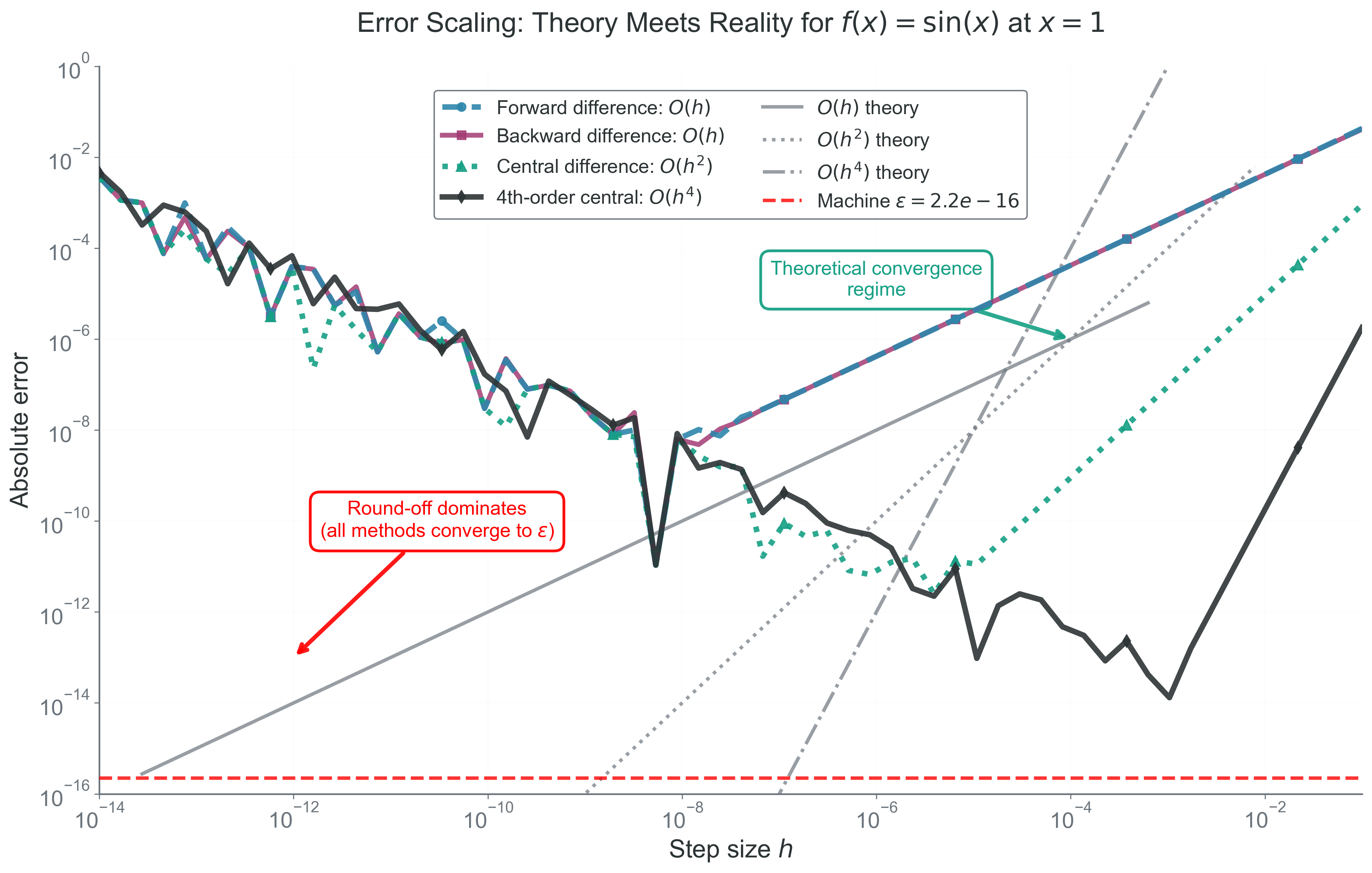
Figure 2:Error scaling comparison for finite difference methods applied to at . Forward (dashed) and backward (solid) differences both show convergence, central difference (dotted) shows , and 4th-order central (solid) shows convergence in the theoretical regime. All methods eventually hit the machine epsilon floor () where round-off dominates. Gray reference lines show exact theoretical scaling.
Implementation: Compact Code Examples
Here’s a minimal implementation of all finite difference methods:
import numpy as np

def finite_diff(f, x, h, method='central'):
    """All finite difference methods in one place"""
    try:
        if method == 'forward':
            return (f(x + h) - f(x)) / h
        elif method == 'backward':
            return (f(x) - f(x - h)) / h
        elif method == 'central':
            return (f(x + h) - f(x - h)) / (2 * h)
        elif method == 'central4':
            return (-f(x+2*h) + 8*f(x+h) - 8*f(x-h) + f(x-2*h)) / (12*h)
        else:
            raise ValueError(f"Unknown method: {method}")
    except (ZeroDivisionError, OverflowError) as e:
raise ValueError(f"Numerical error in {method} difference: {e}")The Fundamental Trade-off: Rigorous Derivation of Optimal 
We’ve established that choosing involves balancing truncation error (from approximating the derivative) and round-off error (from finite precision arithmetic). Let’s now rigorously derive the optimal value of for each method.
Forward Difference: Optimal Step Size
For the forward difference method, we have two sources of error:
Truncation error:
Round-off error:
The total error is:
To find the optimal , we minimize this by taking the derivative with respect to :
Solving for :
For functions where and are of similar magnitude:
This is a remarkable result: even though our numbers have 16 digits of precision, we can only compute derivatives to about 8 digits of accuracy using forward differences!
Central Difference: Even Better Optimal Step Size
For central difference, the error components are:
Truncation error:
Round-off error:
Following the same minimization procedure:
This is crucial: central difference allows a step size that is about 300 times larger than forward difference while achieving better accuracy!
Visualizing the Error Trade-off
Why this matters: The competition between truncation and round-off error creates a fundamental limit on numerical accuracy. This visualization shows why we can’t just make arbitrarily small - there’s an optimal value where total error is minimized. Understanding this trade-off is crucial for choosing appropriate step sizes in your simulations.
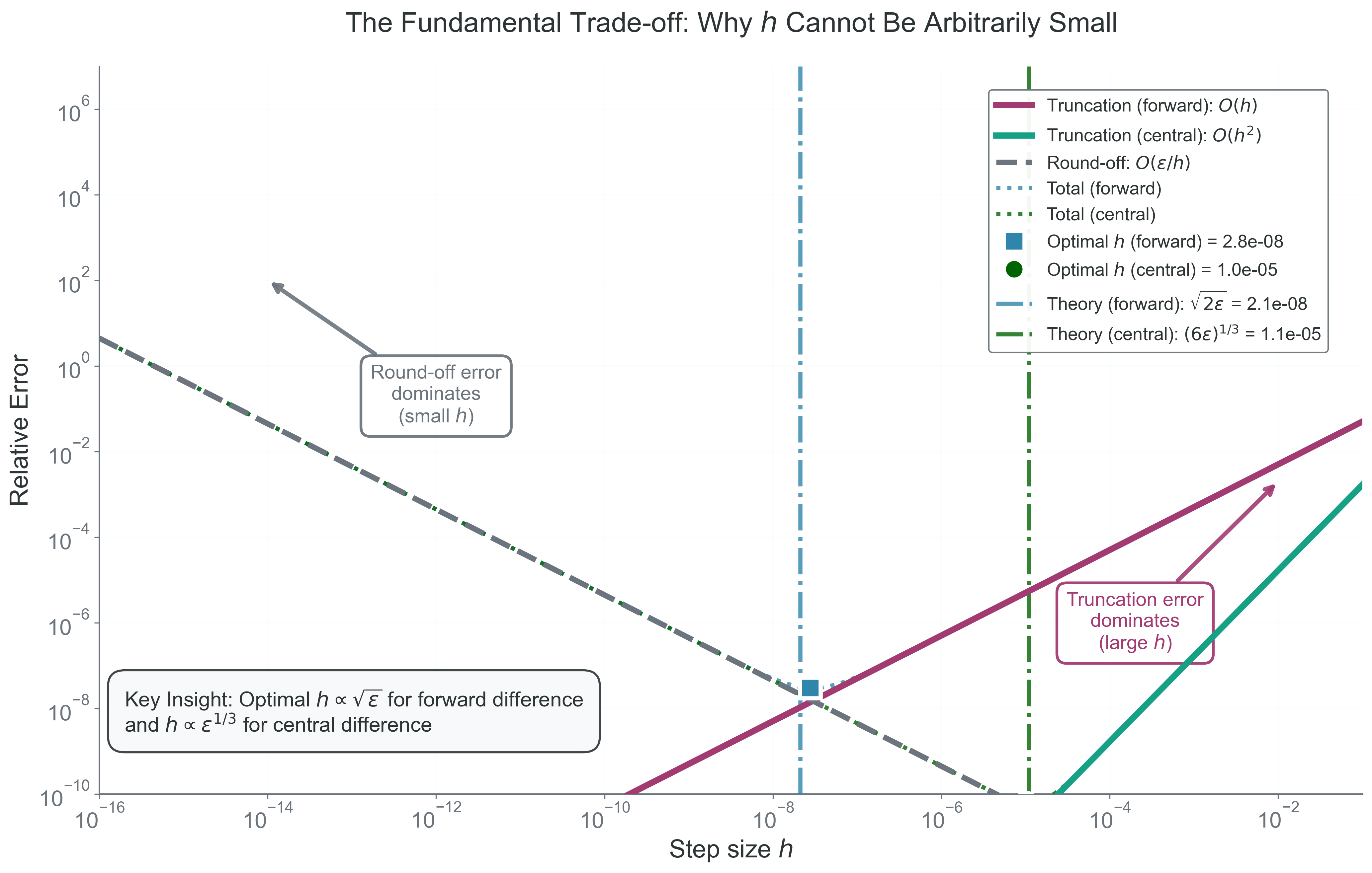
Figure 3:The fundamental trade-off in numerical derivatives showing why cannot be arbitrarily small. Thick lines show component errors: truncation error decreases as for forward differences and for central differences, while round-off error increases as . Total errors (dotted lines) have minima at optimal values: for forward and for central differences.
For large , truncation error dominates. For small , round-off error dominates. The optimal sits at the bottom of the U.
Practical Algorithm for Choosing 
Why this matters: In real applications, you won’t know the derivatives or needed for the theoretical optimal . This practical algorithm estimates appropriate step sizes based on the problem scale and machine precision. This is what you’ll actually use in your research code.
import numpy as np

def practical_optimal_h(x, method='central'):
    """
    Choose h based on method and problem scale

    The key insight: h should scale with |x| to maintain
    relative precision for large values
    """
    epsilon = 2.2e-16

    if abs(x) < epsilon:
        raise ValueError(f"x too close to zero for reliable derivatives")

    x_scale = max(abs(x), 1.0)  # Avoid division issues near zero

    if method in ['forward', 'backward']:
        h_opt = np.sqrt(epsilon) * x_scale
    elif method == 'central':
        h_opt = epsilon**(1/3) * x_scale
    elif method == 'central4':
        h_opt = epsilon**(1/5) * x_scale
    else:
        raise ValueError(f"Unknown method: {method}")

    # Ensure h is not too small relative to x
    h_final = max(h_opt, epsilon * abs(x))
    return h_final

# Example: Choosing h for different problem scales
x_values = [1.0, 1.496e13, 1.989e33]  # dimensionless, 1 AU, 1 M_sun
for x in x_values:
    h = practical_optimal_h(x, 'central')
    print(f"x = {x:.2e}, optimal h = {h:.2e}, h/x = {h/x:.2e}")
Bridge to Part 2: From Derivatives to Machine Arithmetic
You now understand the fundamental paradox: computers cannot take true limits, forcing us to balance truncation and round-off error. But where does this round-off error come from?
In Part 2, we’ll dive deep into how computers represent numbers. You’ll discover:
Why 0.1 + 0.2 ≠ 0.3 in binary arithmetic
How to find and work with machine epsilon
When catastrophic cancellation destroys your calculations
How errors propagate through millions of timesteps
The derivative methods you’ve just learned are built on the foundation of floating-point arithmetic. Understanding this foundation will help you write more robust code and diagnose mysterious numerical failures in your simulations.
Next: Part 2 - Numbers Aren’t Real