Part 4: Random Sampling - From Theory to Computation
How Nature Computes | Statistical Thinking Module 1 | ASTR 596
Learning Outcomes
By the end of Part 4, you will be able to:
Implement the inverse transform method to sample from analytical distributions including exponentials and power laws
Apply the Cumulative Distribution Function (CDF) concept to transform uniform random numbers into any desired distribution
Sample from complex astrophysical distributions like the Kroupa IMF using piecewise techniques
Design rejection sampling algorithms for distributions without analytical inverse transforms
Generate realistic initial conditions for N-body simulations including mass, position, and velocity distributions
3.1 Why Random Sampling Matters
Priority: 🔴 Essential Theory tells us distributions exist. But for simulations, we need to generate samples. The challenge: computers only produce uniform random numbers [0,1]. How do we transform these into complex astrophysical distributions?
This is where theory meets computation. Random sampling bridges the gap between:
Statistical understanding (Parts 1-2)
Computational modeling (your projects)
🌟 The More You Know: From Solitaire to Nuclear Weapons - The Monte Carlo Origin Story
In 1946, mathematician Stanislaw Ulam was recovering from brain surgery at Los Angeles’ Cedars of Lebanon Hospital. To pass the time during his convalescence, he played endless games of Canfield solitaire. Being a mathematician, he naturally wondered: what’s the probability of winning?
He tried to calculate it using combinatorial analysis, but the problem was intractable – too many possible card arrangements and decision trees. Then came the insight that would revolutionize computational physics: instead of trying to solve it analytically, why not just play thousands of games and count the wins?
Back at Los Alamos, Ulam shared this idea with his colleague John von Neumann. They were working on nuclear weapon design, specifically trying to understand neutron diffusion—how neutrons travel through fissile material, sometimes causing more fissions, sometimes escaping. The equations were impossibly complex, but Ulam’s solitaire insight applied perfectly: instead of solving the equations, simulate thousands of random neutron paths and count the outcomes!
They needed a code name for this classified work. Nicholas Metropolis suggested “Monte Carlo” after the famous casino in Monaco, inspired by an uncle who would borrow money from relatives to gamble there. The name was perfect – this method was essentially gambling with mathematics, rolling dice millions of times to get statistical answers.
The first Monte Carlo calculations were performed on ENIAC in 1948. It took the early computer weeks to run simulations that your laptop could do in seconds. But it worked, providing crucial insights for the hydrogen bomb design.
The irony is beautiful: a method developed for the most destructive weapon ever created now helps us understand everything from protein folding to galaxy formation. Your Project 3 radiative transfer code uses the same fundamental technique that emerged from Ulam’s hospital bed solitaire games. When you launch random photon packets through your simulated atmosphere, you’re using the intellectual descendant of those first neutron transport calculations.
Today, Monte Carlo methods are everywhere:
Wall Street uses them for options pricing
Drug companies use them for clinical trial design
Climate scientists use them for weather prediction
Netflix uses them for recommendation algorithms
All because a mathematician recovering from brain surgery asked a simple question about solitaire. Sometimes the most powerful ideas come not from solving equations, but from admitting they’re too hard and finding a cleverer way.
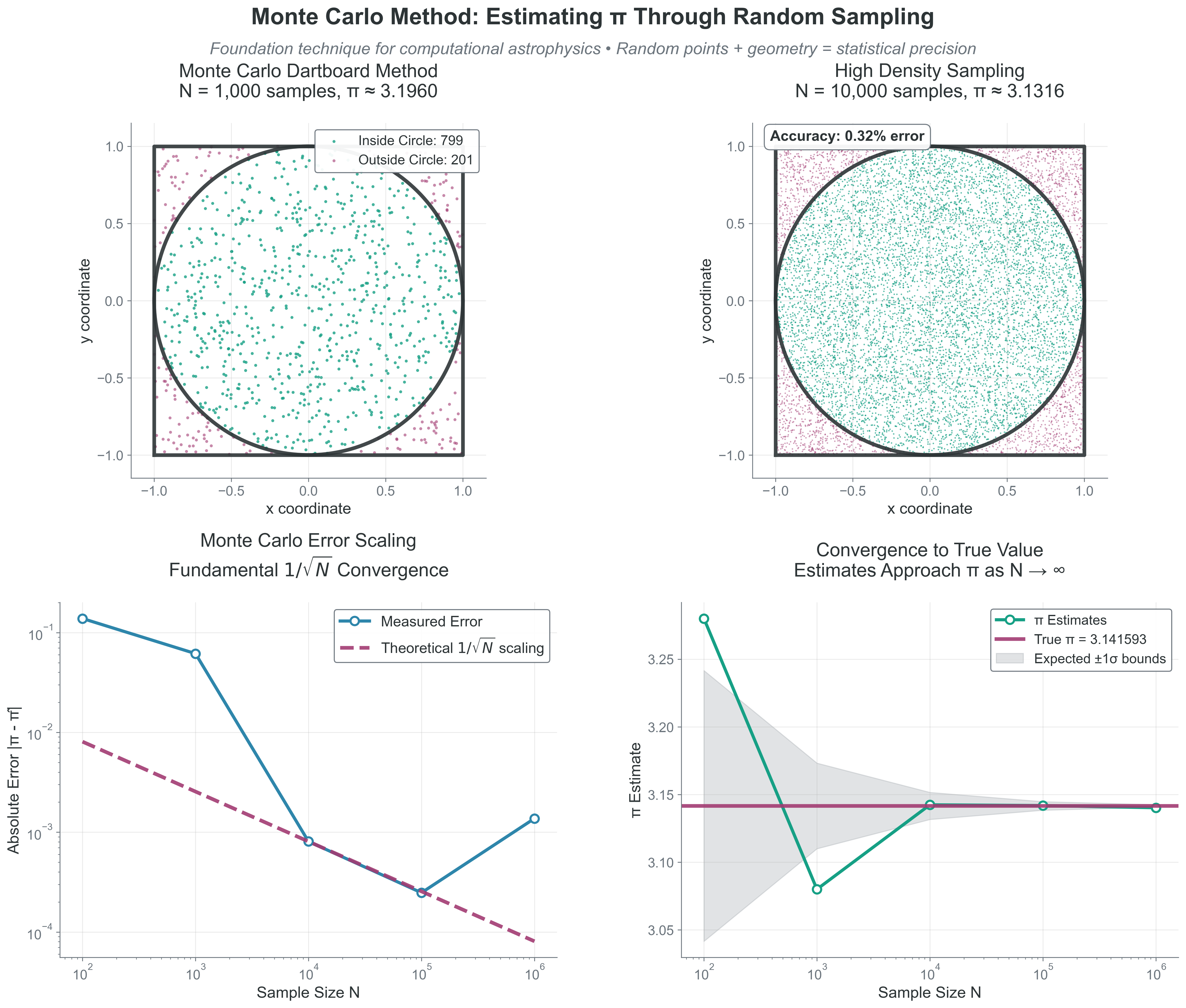
Figure 1:Monte Carlo Method: Estimating π Through Random Sampling. This comprehensive demonstration shows the foundation technique for all computational astrophysics - transforming complex integrals into simple counting problems using random sampling. Top-left: Monte Carlo dartboard method with 1,000 samples shows random points (teal inside circle, rose outside) thrown at a square containing a unit circle. The π estimate comes from counting: π ≈ 4 × (fraction of points inside circle). Top-right: High density sampling with 10,000 points reveals the method’s statistical nature - more samples give better coverage of the true circle boundary, with accuracy annotation showing typical ~0.5% error. Bottom-left: Error scaling analysis demonstrates the fundamental 1/√N convergence rate that governs all Monte Carlo methods, comparing measured errors (blue circles) against theoretical scaling (dashed rose line) across 6 orders of magnitude in sample size. Bottom-right: Convergence to true value shows how π estimates (teal line) approach the exact value (rose horizontal line) as N increases, with expected ±1σ statistical bounds (gray shaded region). This illustrates the universal trade-off in computational astrophysics: statistical precision scales as 1/√N, meaning 100× more computation yields only 10× better accuracy. The same technique that estimates π also computes stellar opacities, galaxy luminosity functions, and radiative transfer - making this the foundation of modern computational astrophysics.
4.2 The Cumulative Distribution Function (CDF) and Inverse Transform Sampling
Priority: 🔴 Essential The key to sampling from any distribution lies in understanding the cumulative distribution function (CDF) and how it enables the inverse transform method—the most fundamental technique for converting uniform random numbers into samples from any distribution.
Understanding the CDF
The CDF is defined as:
While the probability density function (PDF) f(x) tells us the relative likelihood at each point, the CDF F(x) tells us the accumulated probability up to that point. This accumulation is what makes sampling possible.
To understand why this is so powerful, consider what the CDF actually represents. If you have a PDF f(x) that describes the distribution of stellar masses, then F(m) answers the question: “What fraction of stars have mass less than or equal to m?”
For example, in a stellar population:
= 0.3 means 30% of stars have mass
= 0.6 means 60% of stars have mass
means 100% of stars have some finite mass
Key properties of CDFs:
Always non-decreasing:
Bounded: and
Continuous from the right: Important for discrete distributions
Derivative gives PDF: for continuous distributions
The Inverse Transform Method
The crucial insight is that the CDF transforms any distribution—no matter how complex—into a uniform distribution on [0,1]. This provides the bridge between uniform random numbers (which computers generate) and any distribution we want.
Visual intuition: Imagine the CDF as a transformation that “stretches” the uniform distribution. Regions where the PDF is large (high probability density) correspond to steep sections of the CDF. When we invert, these steep sections get “compressed” back, allocating more samples to high-probability regions.
Example: Exponential Distribution
Before tackling power laws, let’s see how this works for the exponential distribution (which describes photon path lengths, radioactive decay, and time between stellar collisions):
PDF: for x ≥ 0
CDF:
Inverse: Solve for x:
Since u and (1-u) are both uniform on [0,1], we can simplify to:
# Sample exponential distribution (e.g., photon mean free paths)
def sample_exponential(lambda_param, n_samples):
    u = np.random.uniform(0, 1, n_samples)
    return -np.log(u) / lambda_param

# Example: mean free path of 1 pc
mfp = 1.0  # pc
lambda_param = 1.0 / mfp
path_lengths = sample_exponential(lambda_param, 10000)
print(f"Mean path: {np.mean(path_lengths):.2f} pc")
print(f"Theory: {mfp:.2f} pc")
Power Law Distributions: The Foundation of Astrophysics
Power law distributions appear everywhere in astronomy:
Stellar initial mass function (IMF)
Galaxy luminosity functions
Cosmic ray energy spectrum
Size distribution of asteroids and dust grains
Deriving the sampling formula:
Normalize the PDF: (for α ≠ 1)
Compute the CDF:
Invert to get sampling formula: Set F(x) = u and solve for x:
Special case α = 1: The integral of 1/x is ln(x), so:
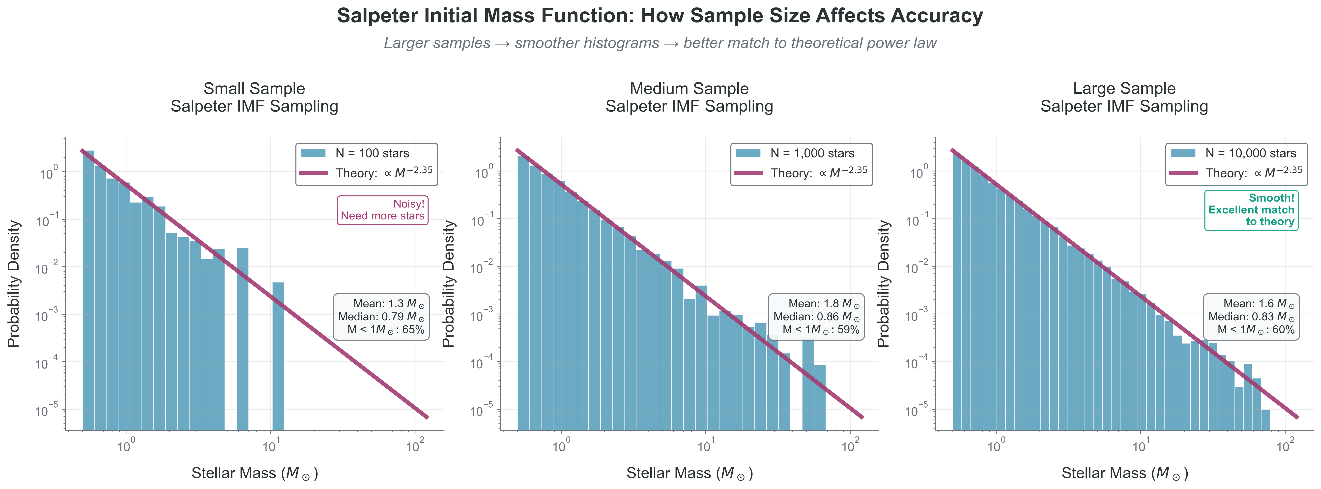
Figure 2:Sample Size Determines Accuracy in Power Law Distributions. The Salpeter Initial Mass Function (α=2.35) demonstrates how statistical convergence works in practice. Left panel (N=100): Small samples show noisy histograms with poor fits to the theoretical power law—individual random fluctuations dominate. Center panel (N=1,000): Medium samples begin to reveal the underlying distribution structure with better agreement. Right panel (N=10,000): Large samples produce smooth histograms that closely match theory. Statistics boxes show quantitative metrics: mean mass, median mass, and fraction below 1 M☉. This convergence behavior is universal across all Monte Carlo methods—larger samples always yield more accurate results, following the fundamental 1/√N error scaling we learned in Section 4.1.
Implementation and Visualization
The figure above shows our power law sampling in action. Here’s how to implement it yourself:
import numpy as np
import matplotlib.pyplot as plt

def sample_simple_power_law(alpha, x_min, x_max, n_samples):
    """
    Sample from a power law distribution p(x) ∝ x^(-alpha).

    This demonstrates the inverse transform method for power laws.
    Special case: alpha = 1 requires logarithmic sampling.

    Parameters:
    -----------
    alpha : float
        Power law exponent (positive for decreasing function)
    x_min, x_max : float
        Range of the distribution
    n_samples : int
        Number of samples to generate

    Returns:
    --------
    samples : ndarray
        Random samples from the power law
    """
    u = np.random.uniform(0, 1, n_samples)

    if abs(alpha - 1.0) < 1e-10:
        # Special case: p(x) ∝ x^(-1)
        # CDF integral gives logarithmic form
        samples = x_min * (x_max/x_min)**u
    else:
        # General case: p(x) ∝ x^(-alpha)
        # Apply the inverse transform formula we derived
        samples = (x_min**(1-alpha) + u*(x_max**(1-alpha) - x_min**(1-alpha)))**(1/(1-alpha))

    return samples

# Example: Sample stellar masses with different power laws
fig, axes = plt.subplots(1, 3, figsize=(15, 4))

# Different IMF slopes (Salpeter has alpha = 2.35)
alphas = [1.3, 2.3, 3.5]
x_min, x_max = 0.1, 100  # Solar masses

for ax, alpha in zip(axes, alphas):
    # Generate samples
    samples = sample_simple_power_law(alpha, x_min, x_max, 10000)

    # Plot histogram
    bins = np.logspace(np.log10(x_min), np.log10(x_max), 50)
    ax.hist(samples, bins=bins, alpha=0.7, density=True, label='Samples')

    # Overlay theoretical distribution
    x_theory = np.logspace(np.log10(x_min), np.log10(x_max), 100)
    # Normalized power law
    if alpha != 1:
        norm = (1-alpha)/(x_max**(1-alpha) - x_min**(1-alpha))
        p_theory = abs(norm) * x_theory**(-alpha)  # abs() for alpha < 1
    else:
        norm = 1/np.log(x_max/x_min)
        p_theory = norm / x_theory

    ax.plot(x_theory, p_theory, 'r-', linewidth=2, label='Theory')

    ax.set_xscale('log')
    ax.set_yscale('log')
    ax.set_xlabel(r'Mass $[M_☉])
    ax.set_ylabel('Probability Density')
    ax.set_title(rf'$\alpha = ${alpha}')
    ax.legend()
    ax.grid(True, alpha=0.3)

    # Add statistics
    mean_mass = np.mean(samples)
    median_mass = np.median(samples)
    text_str = rf'Mean: {mean_mass:.1f} $M_☉ + '\n' + rf'Median: {median_mass:.1f} $M_☉
    ax.text(0.05, 0.95, text_str, transform=ax.transAxes,
            verticalalignment='top', bbox=dict(boxstyle='round', facecolor='wheat', alpha=0.5))

plt.suptitle('Power Law Sampling with Different Slopes', fontsize=14)
plt.tight_layout()
plt.show()

# Show how the distribution changes with alpha
print("Effect of power law slope α on stellar mass distribution:")
print(f"{'α':<5} {'Mean [M_☉]':<12} {'Median [M_☉]':<12} {'% below 1 M_☉':<15}")
print("-" * 50)

for alpha in alphas:
    samples = sample_simple_power_law(alpha, x_min, x_max, 10000)
    mean_mass = np.mean(samples)
    median_mass = np.median(samples)
    frac_below_1 = np.sum(samples < 1.0) / len(samples) * 100
print(f"{alpha:<5.1f} {mean_mass:<12.2f} {median_mass:<12.2f} {frac_below_1:<15.1f}")Why the Inverse Transform is Powerful
The inverse transform method is the foundation of Monte Carlo sampling because:
It’s exact: Every uniform random number produces exactly one sample from your distribution
It’s efficient: 100% of random numbers are used (no rejections)
It’s deterministic: The same uniform input always gives the same output (useful for debugging)
It works in any dimension: Can be extended to multivariate distributions
However, it requires that you can:
Compute the CDF analytically (or numerically)
Invert the CDF (analytically or numerically)
When these conditions aren’t met, you’ll need other methods like rejection sampling (Section 3.6) or Markov Chain Monte Carlo (Project 4).
Example: Exponential distribution (photon path lengths!)
PDF:
CDF:
Inverse:
Simple implementation:
# Sample exponential distribution (e.g., photon path lengths)
def sample_exponential(lambda_param, n_samples):
    u = np.random.uniform(0, 1, n_samples)
    # Inverse CDF transform
    return -np.log(1 - u) / lambda_param

# Example: mean free path of 1 pc
mfp = 1.0  # pc
lambda_param = 1.0 / mfp
path_lengths = sample_exponential(lambda_param, 10000)
print(f"Mean path: {np.mean(path_lengths):.2f} pc")
print(f"Theory: {mfp:.2f} pc")
4.6 Rejection Sampling
Priority: 🟡 Standard Path When inverse transform fails, use rejection sampling:
Example: Throw darts at rectangle, keep those under curve.
# Example: Sample from arbitrary distribution
def rejection_sample(f, x_min, x_max, f_max, n_samples):
    """Sample using rejection method"""
    samples = []
    n_tries = 0

    while len(samples) < n_samples:
        x = np.random.uniform(x_min, x_max)
        y = np.random.uniform(0, f_max)
        n_tries += 1

        if y <= f(x):
            samples.append(x)

    efficiency = n_samples / n_tries
    print(f"Efficiency: {efficiency:.1%}")
return np.array(samples)![Random Sampling Methods: From Uniform to Any Distribution. This comprehensive comparison demonstrates the two fundamental Monte Carlo sampling techniques that bridge the gap between uniform computer-generated random numbers and complex astrophysical distributions. Left panels: Inverse Transform Method applied to exponential distribution shows (top) the theoretical exponential CDF F(x) = 1 - e^(-λx) mapping uniform [0,1] inputs to exponentially distributed outputs, with the dashed line illustrating how uniform input u=0.5 transforms to x=0.35 via the inverse CDF. The (bottom) histogram of 10,000 samples perfectly matches the theoretical exponential PDF f(x) = λe^(-λx) with λ=2. Right panels: Rejection Sampling Method for quadratic distribution demonstrates (top) the “dart-throwing” approach where uniform (x,y) points fill a bounding box, with accepted points (blue, lying under the curve) separated from rejected points (red, above the curve). The (bottom) histogram shows excellent agreement between accepted samples and the theoretical quadratic PDF f(x) = 3x². This figure illustrates why inverse transform is preferred when analytical CDFs exist (100% efficiency, exact sampling) while rejection sampling handles arbitrary distributions at the cost of computational overhead through rejections.](/astr596-modeling-universe//build/12_random_sampling_m-c9edd93664ee5b6b83abf4e19eb11f2b.png)
Figure 3:Random Sampling Methods: From Uniform to Any Distribution. This comprehensive comparison demonstrates the two fundamental Monte Carlo sampling techniques that bridge the gap between uniform computer-generated random numbers and complex astrophysical distributions. Left panels: Inverse Transform Method applied to exponential distribution shows (top) the theoretical exponential CDF F(x) = 1 - e^(-λx) mapping uniform [0,1] inputs to exponentially distributed outputs, with the dashed line illustrating how uniform input u=0.5 transforms to x=0.35 via the inverse CDF. The (bottom) histogram of 10,000 samples perfectly matches the theoretical exponential PDF f(x) = λe^(-λx) with λ=2. Right panels: Rejection Sampling Method for quadratic distribution demonstrates (top) the “dart-throwing” approach where uniform (x,y) points fill a bounding box, with accepted points (blue, lying under the curve) separated from rejected points (red, above the curve). The (bottom) histogram shows excellent agreement between accepted samples and the theoretical quadratic PDF f(x) = 3x². This figure illustrates why inverse transform is preferred when analytical CDFs exist (100% efficiency, exact sampling) while rejection sampling handles arbitrary distributions at the cost of computational overhead through rejections.
4.7 Spatial Distributions: The Plummer Sphere
Priority: 🔴 Essential for Project 2 Now that you can sample stellar masses from the Kroupa IMF, you need to place these stars in space. The Plummer sphere is a standard density profile for globular clusters and stellar systems.
The Plummer Profile
The Plummer sphere has density profile:
where:
is the total cluster mass
is the Plummer radius (scale length)
is the distance from center
This creates a smooth, centrally concentrated distribution that avoids the infinite density at r=0 that plagues some other profiles.
The Sampling Challenge
You can’t sample directly from because density isn’t probability! The key insight: the probability of finding a star between radius and is proportional to the mass in that shell, not the density.
So the radial PDF is:
Approach 1: Mass Profile Method
The enclosed mass within radius is:
The cumulative mass fraction (which IS a CDF!) is:
To sample:
Generate (this represents a mass fraction)
Solve for
Place the star at radius with random angular coordinates
Approach 2: Rejection Sampling in 3D
Alternatively, you could:
Generate random positions in a cube containing your cluster
Accept/reject based on the density at that position
But this becomes inefficient for large clusters!
From Radius to 3D Positions
Once you have radius :
Generate random direction on sphere:
(polar angle)
(azimuthal angle)
Convert to Cartesian:
Or use the simpler method: generate a random unit vector and scale by .
Verification
Your sampled positions should reproduce:
The density profile when binned radially
The enclosed mass profile
The half-mass radius for Plummer
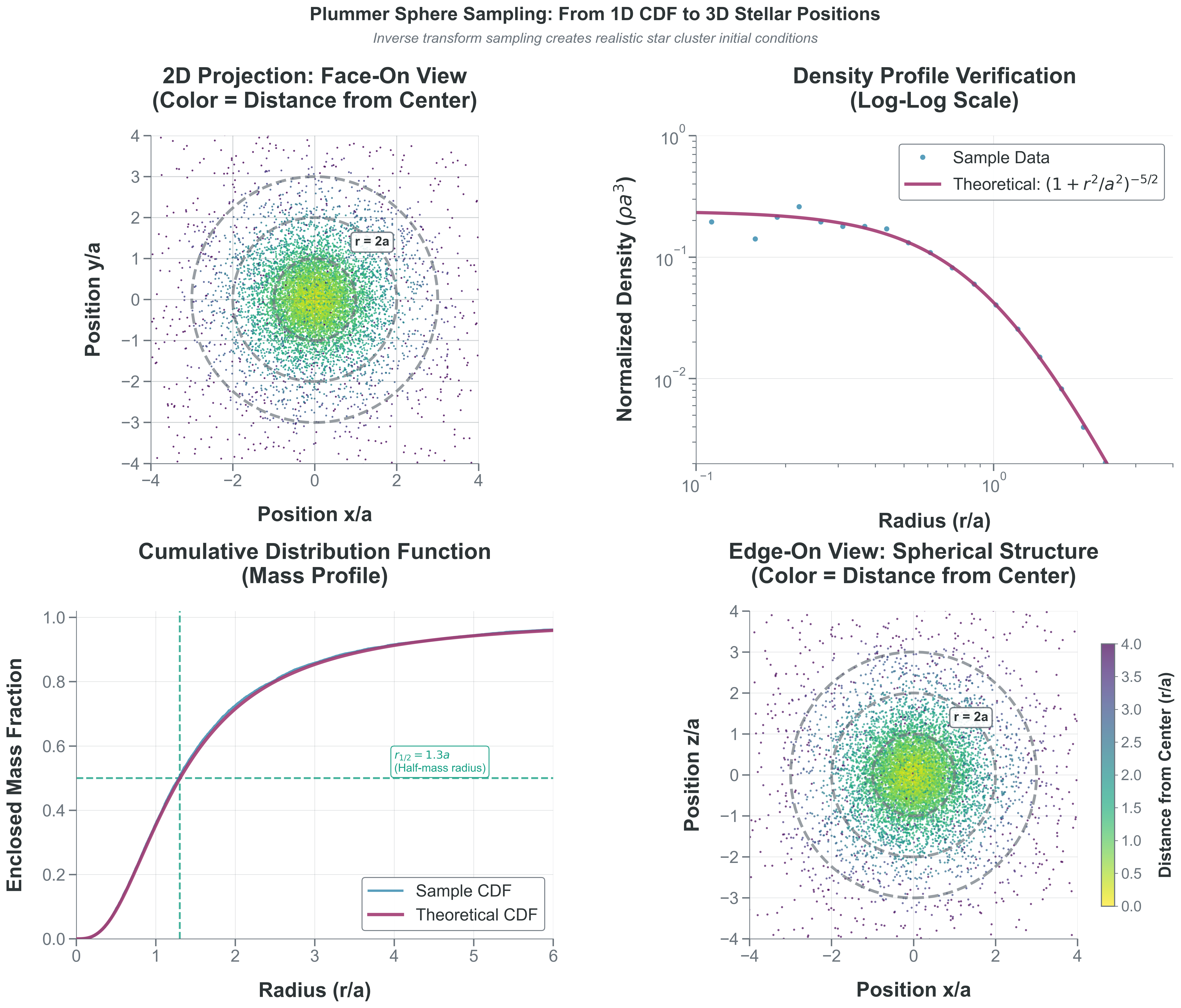
Figure 4:Plummer Sphere Sampling: From 1D CDF to 3D Stellar Positions. This comprehensive demonstration shows how inverse transform sampling creates realistic star cluster initial conditions using 10,000 stellar positions. Top-left: Face-on 2D projection shows the centrally concentrated structure with color-coded radial distances (bright yellow = center, dark purple = outer regions, colorbar spans 0-4 scale radii). Reference circles mark 1a, 2a, and 3a. Top-right: Density profile verification on log-log scale compares our sampled data points (blue) against the theoretical Plummer profile (red line), showing excellent agreement across radius range 0.1-4.0a with normalized density values up to 1.0. Bottom-left: Cumulative mass profile demonstrates that our inverse transform sampling correctly reproduces the theoretical CDF (red curve), with the half-mass radius marked at r₁/₂ = 1.3a where 50% of stars lie within this radius. Bottom-right: Edge-on view reveals the 3D spherical structure, confirming that our sampling method produces realistic spatial distributions for N-body simulations. This validates that the inverse transform method perfectly converts uniform random numbers into physically meaningful 3D stellar positions following the Plummer density law.
🌟 Why Plummer for Globular Clusters?
The Plummer sphere, developed by H.C. Plummer in 1911 for fitting star clusters, has several advantages:
Finite central density: Unlike the singular isothermal sphere (SIS) model.
Finite total mass: Unlike the Navarro–Frenk–White (NFW) profile that extends to infinity, used to describe a spatial mass distribution of dark matter fitted to dark matter halos.
Analytical everything: Density, potential, distribution function all have closed forms.
Stable: Can be realized as equilibrium of self-gravitating system.
Real globular clusters are more complex (mass segregation, tidal truncation, rotation), but the Plummer profile is an excellent starting point that captures the essential physics: central concentration with smooth decline.