Part 1: Root Finding - Where Physics Reaches Equilibrium
Static Problems & Quadrature | Numerical Methods Module 2 | ASTR 596
Learning Outcomes
By the end of this section, you will be able to:
Implement bisection, Newton-Raphson, and secant methods from scratch
Analyze convergence rates (linear, superlinear, quadratic) mathematically
Diagnose method failures and design robust hybrid approaches
Apply root finding to Kepler’s equation, Lagrange points, and stellar structure
Predict iteration counts and verify convergence behavior
The Fundamental Problem
In physics, equilibrium occurs where the net force vanishes, where energy is minimized, or where competing effects balance. Mathematically, these all reduce to finding roots of equations: solving .
But here’s the challenge: most astrophysical equations are transcendental equations that cannot be solved analytically. Consider finding where a star’s pressure balances gravity:
With realistic equations of state and composition gradients, this becomes a transcendental equation with no closed-form solution. We need numerical methods.
Building Intuition: The Geometry of Root Finding
Before diving into algorithms, let’s understand the geometry. Finding roots is about discovering where a curve crosses the x-axis. Different methods use different geometric insights:
Bracketing methods (Bisection): Trap the root between two points and squeeze—when you absolutely must find the root, even if slowly
Local approximation methods (Newton): Follow the tangent line to the axis—when you need maximum speed and have derivatives
Interpolation methods (Secant): Approximate the curve with simpler functions—the practical compromise when derivatives are expensive
Each approach has trade-offs between:
Reliability: Will it always find a root?
Speed: How many iterations to converge?
Requirements: Do we need derivatives? Good initial guesses?
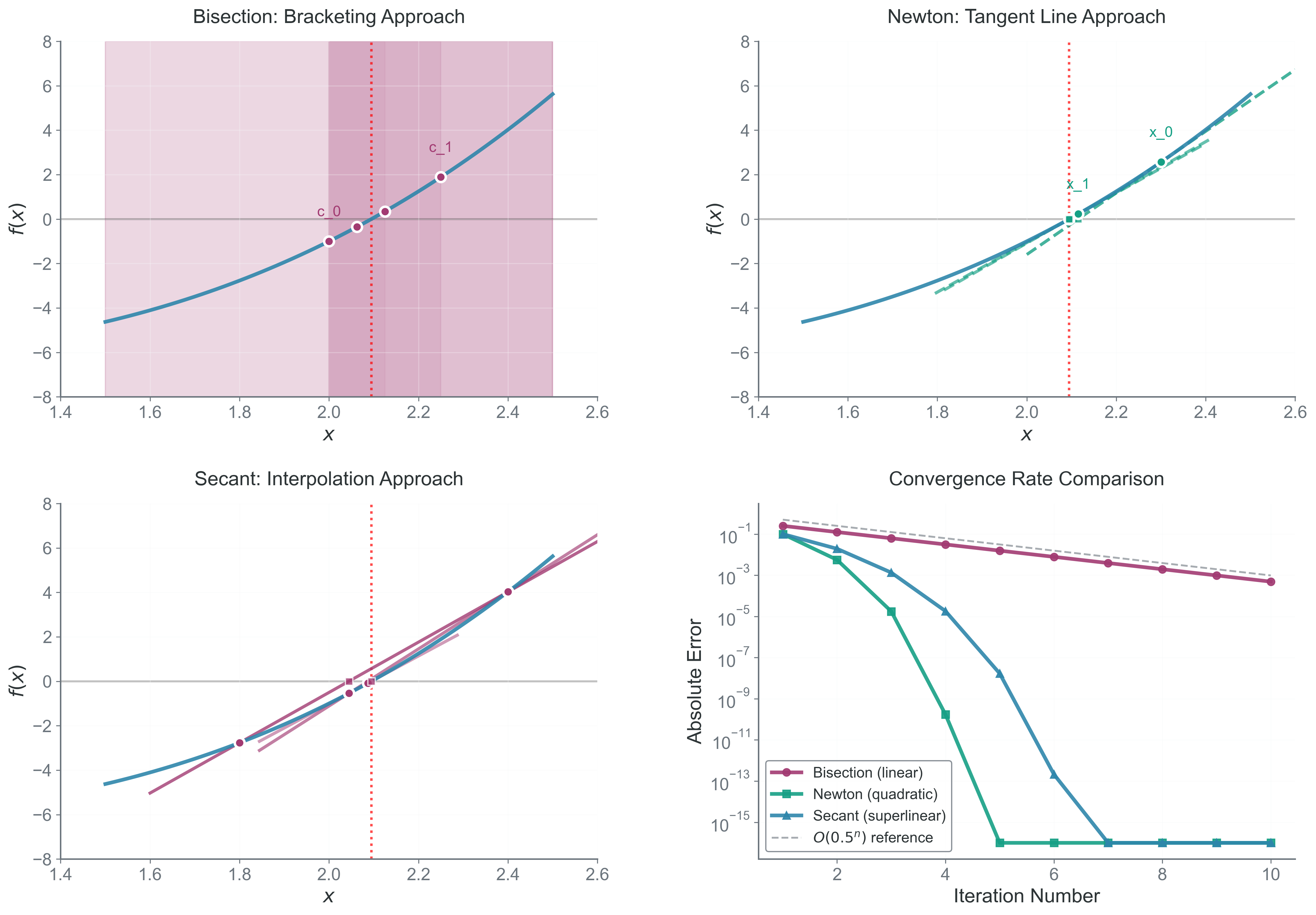
Figure 1:Three geometric approaches to root finding. The top panels show how bisection (bracketing), Newton (tangent lines), and secant (interpolation) methods work geometrically on the function . The bottom-right convergence plot reveals the mathematical power of each approach: bisection’s reliable but slow linear convergence, secant’s faster superlinear convergence, and Newton’s rapid quadratic convergence when conditions are favorable. Note how the different slopes on the log-scale plot correspond to different convergence orders—a key signature for identifying method performance in practice.
Method 1: Bisection - The Reliable Workhorse
The Mathematical Foundation
The bisection method is based on the Intermediate Value Theorem:
If is continuous on and , then there exists at least one root where .
The algorithm repeatedly halves the interval, keeping the half that contains the root.
Algorithm Analysis
Starting with interval where :
Compute midpoint:
Evaluate
Update interval:
If : Found root to desired accuracy
If : root in , so set ,
Otherwise: root in , so set ,
After iterations, the interval width is:
The error in our approximation is bounded by half the interval width:
This is linear convergence with rate .
Iterations Required
To achieve error , we need:
Solving for :
For example, to find a root in to 10 decimal places ():
So we need 33 iterations—slow but guaranteed!
Implementation
Here’s a complete bisection implementation to understand the algorithm:
def bisection(f, a, b, tol=1e-10, max_iter=100):
    """Find root of f in [a,b] by bisection"""
    # Check initial bracket
    fa, fb = f(a), f(b)
    if fa * fb >= 0:
        raise ValueError("Need f(a) and f(b) with opposite signs")
    if abs(fa) < tol: return a
    if abs(fb) < tol: return b

    for i in range(max_iter):
        c = (a + b) / 2
        fc = f(c)

        if abs(fc) < tol or abs(b - a) < 2*tol:
            return c

        if fa * fc < 0:
            b, fb = c, fc
        else:
            a, fa = c, fc

    raise RuntimeError(f"Failed to converge in {max_iter} iterations")
Common Failure Modes and Fixes
| Problem | Symptom | Solution |
|---|---|---|
| No sign change | Won’t start | Scan interval for brackets first |
| Multiple roots | Finds arbitrary one | Use smaller initial intervals |
| Discontinuity | False bracket | Check continuity requirement |
| f touches zero | No sign change | Use f²(x) which has same roots |
Method 2: Newton-Raphson - The Speed Demon
The Geometric Insight
Newton’s method uses calculus to accelerate convergence. The key insight: near any point, a smooth function looks approximately linear. We can follow the tangent line to where it crosses the axis, getting much closer to the root in a single step.
Mathematical Derivation
Starting at point , the tangent line to has equation:
This line crosses the x-axis (where ) at:
Solving for :
This is the Newton-Raphson iteration formula.
Convergence Analysis
To understand the convergence rate, we analyze the error where is the true root.
Using Taylor series around :
Since :
Similarly:
Through algebraic manipulation of the Newton iteration formula:
This shows quadratic convergence! The error is squared each iteration, meaning the number of correct digits approximately doubles.
When Newton Fails
Despite its speed, Newton’s method can fail spectacularly:
Zero derivative: If , the tangent is horizontal and never crosses the axis
Poor initial guess: May diverge or converge to wrong root
Cycles: Can oscillate between points without converging
Ill-conditioned: When is very small, round-off errors dominate
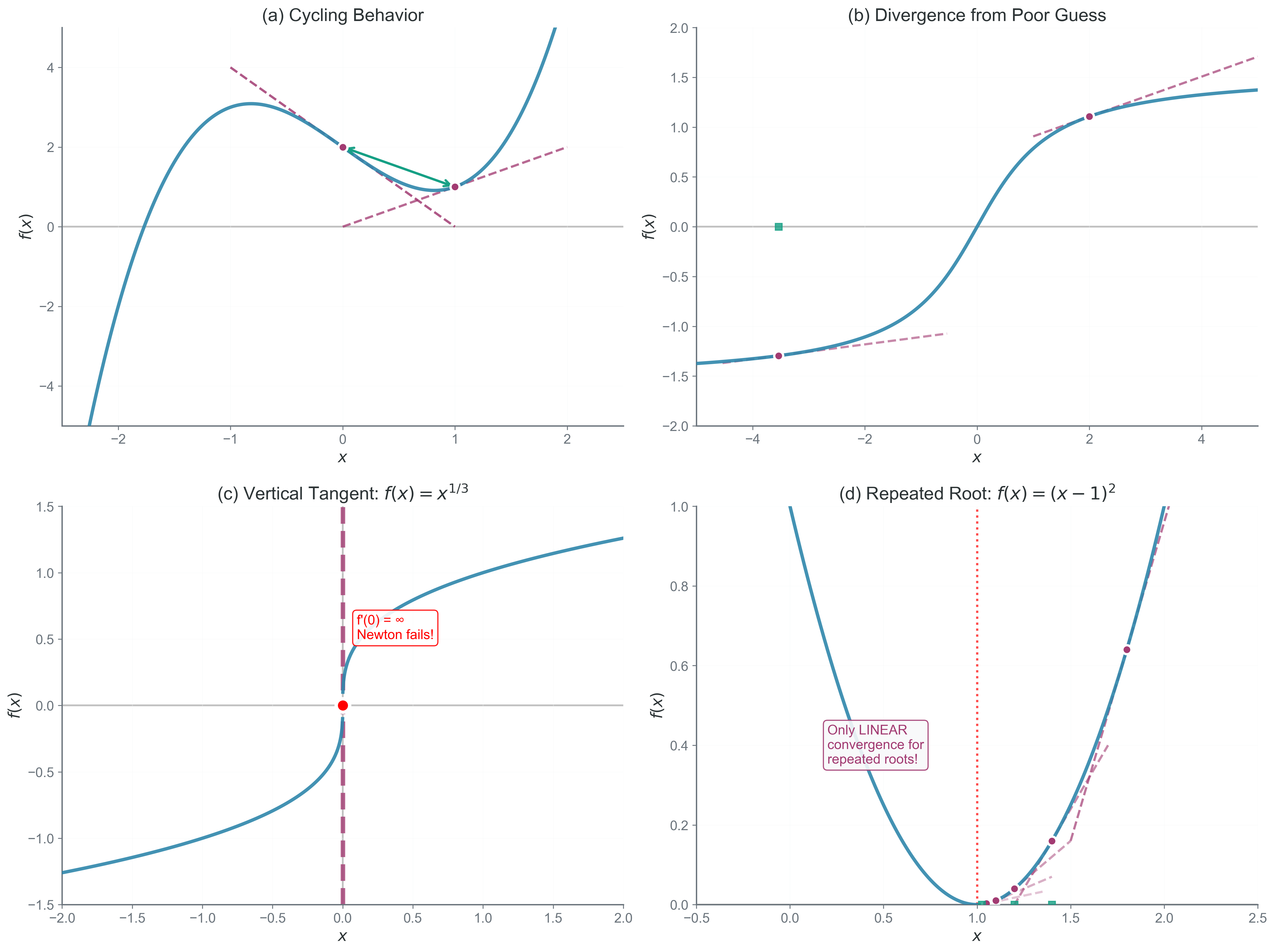
Figure 2:When Newton’s method fails. Four critical failure modes illustrate why Newton’s method, despite its speed, requires careful application: (a) Cycling behavior occurs when iterates bounce between points without converging; (b) Divergence from poor initial guesses sends the method away from the root; (c) Vertical tangents (infinite derivatives) cause division by zero; (d) Repeated roots reduce convergence from quadratic to merely linear. Understanding these failure patterns is essential for robust algorithm design—they explain why production codes often combine Newton with bracketing methods for reliability.
Common Failure Modes and Fixes
| Problem | Symptom | Solution |
|---|---|---|
| f’(x) ≈ 0 | Division by small number | Switch to bisection |
| Bad initial guess | Divergence | Use bisection to bracket first |
| Oscillation | Repeating values | Detect cycles, switch methods |
| Repeated root | Slow convergence | Use modified Newton: |
Method 3: Secant - The Practical Compromise
Motivation: No Derivatives Required
Newton’s method requires , but what if:
The derivative is expensive to compute?
We only have as a black box?
The function comes from experimental data?
The secant method approximates the derivative using a finite difference:
The Iteration Formula
Substituting this approximation into Newton’s formula:
Geometrically, we’re replacing the tangent line with a secant line through two points.
Convergence Analysis
The convergence of the secant method is more complex. Through detailed analysis (involving difference equations), one can show that the order of convergence is:
This is the golden ratio! The error satisfies:
This superlinear convergence is slower than Newton’s quadratic rate but faster than bisection’s linear rate.
Comparison of Convergence Rates
| Method | Order | Error Reduction | Digits Gained/Iteration | Function Evals |
|---|---|---|---|---|
| Bisection | 1.0 | 0.30 | 1 | |
| Secant | 1.618 | ~0.62 | 1 | |
| Newton | 2.0 | Doubles | 2 (f and f’) |
Common Failure Modes and Fixes
| Problem | Symptom | Solution |
|---|---|---|
| f(x₀) ≈ f(x₁) | Near-zero denominator | Perturb one point slightly |
| Parallel secants | No convergence | Restart with different points |
| Leaves bracket | May miss root | Combine with bisection (Brent’s method) |
Hybrid Methods: Best of All Worlds
In practice, we often combine methods to leverage their strengths:
Brent’s Method
Combines bisection’s reliability with inverse quadratic interpolation’s speed:
Maintains a bracketing interval like bisection
Tries fast interpolation when possible
Falls back to bisection if interpolation fails
Never worse than bisection, often much faster
Practical Strategy for Robust Root Finding
1. Start with bisection to bracket the root
2. Switch to Newton/Secant once close enough
3. Fall back to bisection if Newton diverges
4. Monitor condition number throughout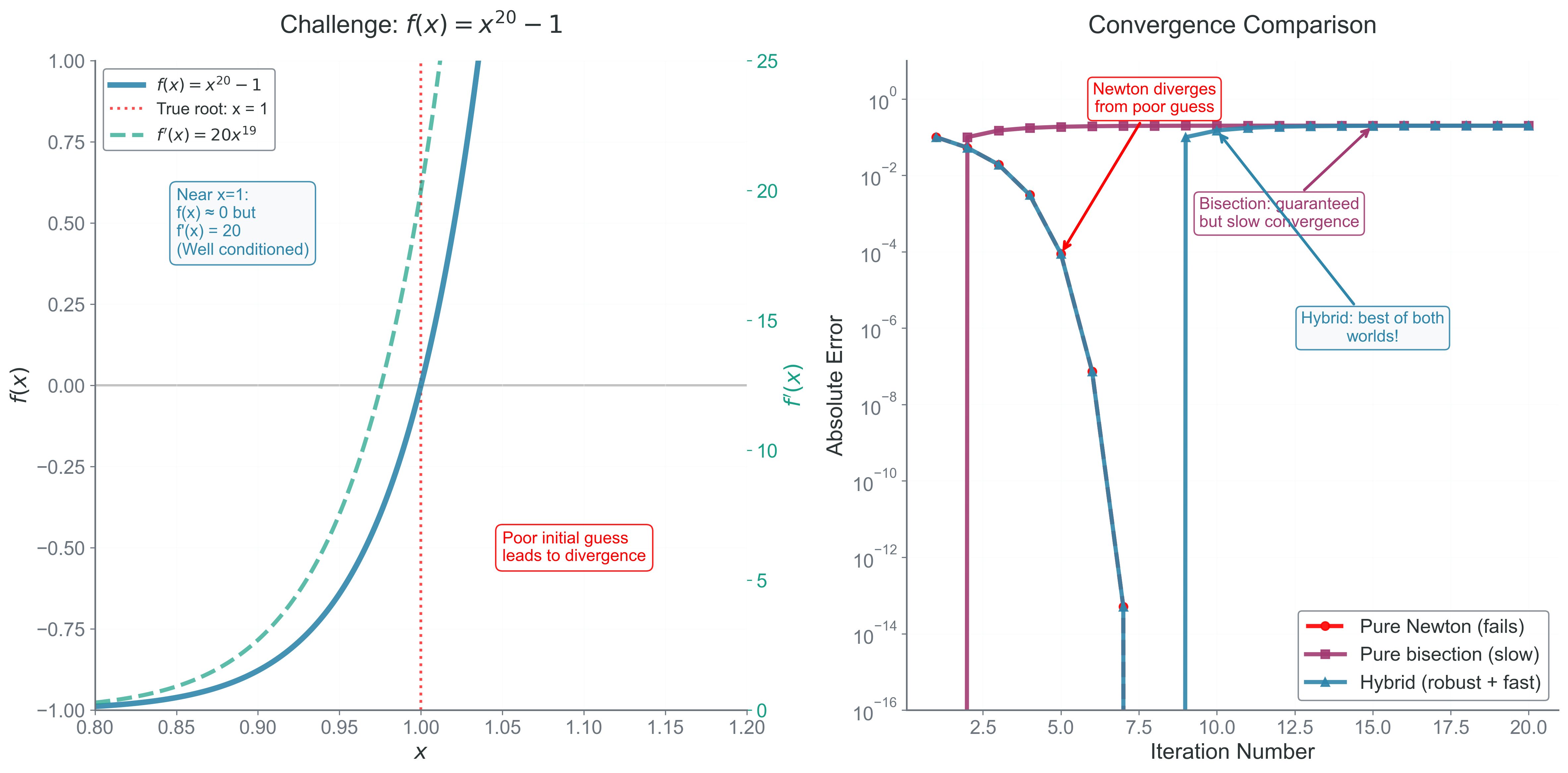
Figure 3:Why production codes use hybrid methods. Testing on the challenging function near reveals the power of combining methods. Pure Newton (red) fails catastrophically from poor initial guesses due to the extreme conditioning of this function. Pure bisection (pink) is reliable but painfully slow, requiring dozens of iterations. The hybrid approach (blue) intelligently switches between methods: it uses bisection to establish a safe bracket, then switches to Newton for rapid final convergence, falling back to bisection if Newton steps become unreliable. This adaptive strategy delivers both robustness and speed—explaining why sophisticated root-finding libraries like those in SciPy implement such hybrid algorithms.
Application: Units and Scaling
Always non-dimensionalize your equations before root finding. Working with rather than improves numerical stability:
Bad: Finding radius where g/cm³ with in cm Good: Define , and solve
This keeps all numbers near unity, avoiding overflow/underflow and improving conditioning.
Physical Example: Stellar Structure Equilibrium
In stellar interiors, hydrostatic equilibrium requires:
For a polytrope with , the Lane-Emden equation describes stellar structure:
where is dimensionless radius and is related to density.
The stellar surface occurs where —a root-finding problem!
For different polytropic indices:
(constant density): exactly
(isothermal core):
(Eddington standard model):
(minimum mass star): (infinite radius!)
Newton’s method excels here because we can compute and from the differential equation. The convergence is rapid even for the sensitive case.
Worked Example: Kepler’s Equation
The most famous root-finding problem in astronomy is Kepler’s equation, which relates mean anomaly (proportional to time) to eccentric anomaly (related to position):
where is the orbital eccentricity and both and are in radians.
Why This Is Hard
Transcendental equation (no algebraic solution)
Must be solved millions of times in orbit propagation
High eccentricity makes convergence difficult
Conditioning worsens as (parabolic orbit)
Newton’s Method Applied
Define
Then
Newton iteration:
Note: when , which can happen for high eccentricity!
Initial Guess Strategy
Good initial guesses are crucial:
For : Use (nearly circular)
For : Use (highly eccentric)
Convergence Analysis
| Eccentricity | Iterations (typical) | Condition Number | Why |
|---|---|---|---|
| 0.0 (circle) | 0 | 1 | E = M exactly |
| 0.1 | 2-3 | ~1.1 | Nearly linear problem |
| 0.5 | 3-4 | ~2 | Moderate nonlinearity |
| 0.9 | 5-7 | ~10 | Strong nonlinearity |
| 0.99 | 10-15 | ~100 | Near-parabolic, poorly conditioned |
Practical Algorithm for Finding Initial Brackets
To find initial brackets for bisection:
def find_brackets(f, x_min, x_max, n_scan=100):
    """Scan interval for sign changes"""
    dx = (x_max - x_min) / n_scan
    brackets = []

    x_prev = x_min
    f_prev = f(x_prev)

    for i in range(1, n_scan + 1):
        x = x_min + i * dx
        fx = f(x)

        if f_prev * fx < 0:
            brackets.append([x_prev, x])

        x_prev, f_prev = x, fx

    return brackets
Debugging Root Finding
Common root-finding bugs and their diagnosis:
| Symptom | Likely Cause | Fix |
|---|---|---|
| Bisection won’t start | Same sign at endpoints | Scan for sign changes first |
| Newton diverges | Poor initial guess or | Use bisection first to bracket |
| Secant oscillates | Nearly parallel secant lines | Check threshold |
| Wrong root found | Multiple roots in region | Narrow search interval |
| Infinite loop | Tolerance too small | Use relative tolerance: |
| No convergence | Discontinuous function | Check function continuity |
Bridge to Part 2: From Finding Zeros to Measuring Areas
You now command three powerful methods for finding where functions equal zero. Each has its place: bisection for reliability, Newton for speed, secant for practicality.
But finding equilibrium points is only half the story. Next, we tackle integration—measuring quantities across space and time. You’ll discover how the same principles of approximation and error analysis apply to computing areas under curves, volumes of regions, and integrals over high-dimensional spaces.
The connection runs deep: integration is the inverse of differentiation, and many integration methods rely on root finding. The error analysis skills you’ve developed here will guide your understanding of quadrature methods.
Next: Part 2 - Quadrature