Part I: The Hidden Physics in Every Astronomical Image
Why the Universe Looks the Way It Does | Statistical Thinking Module 4 | ASTR 596
Learning Objectives
By the end of Part I, you will be able to:
Explain how photon energy relates to physical processes through
Calculate extinction effects on stellar observations using
Quantify wavelength-dependent extinction and its impact on astronomical observations
Connect different wavelengths to their underlying physical processes and temperatures
Apply extinction corrections to determine true stellar distances and properties
Recognize that astronomical images encode physics through photon energies and wavelengths
Part I: The Hidden Physics in Every Astronomical Image
“The nitrogen in our DNA, the calcium in our teeth, the iron in our blood, the carbon in our apple pies were made in the interiors of collapsing stars. We are made of starstuff.”
Carl Sagan
From Pretty Pictures to Profound Physics
You probably fell in love with astronomy through astronomical images – the ethereal Horsehead Nebula silhouetted against glowing gas, the jeweled splendor of the Orion Nebula, the delicate veils of the Veil Nebula. These images move us in ways that equations never could. But here’s what your introductory astronomy course might not have emphasized: those gorgeous colors aren’t just aesthetic choices by image processors. Every hue, every shadow, every glowing wisp is physics speaking to us across cosmic distances. Each photon that reaches our telescopes carries a story – a story of its birth in stellar furnaces or shocked gas, a story of its journey through cosmic dust and gas, and crucially, a story of its missing companions who never made it to our detectors.
The reddish glow of a nebula? That’s hydrogen atoms cascading down energy levels at precisely 656.28 nanometers (nm = 10-7 cm), releasing exactly 1.89 eV of energy per photon.
The dark lanes cutting through star fields? That’s submicron-sized ( cm) interstellar dust grains filtering starlight.
The fact that JWST sees thousands of stars where Hubble sees only darkness? That’s infrared light navigating through obstacles that block visible wavelengths.
![Rubin Observatory’s First Light on the Lagoon and Trifid Nebulae. This iconic first-release image from the Rubin Observatory captures the vivid interplay of nebulae, dust, and star clusters in Sagittarius. Notice how the rich reds and pinks trace hydrogen-alpha emission (656 nm), pinpointing regions of active star formation and ionized gas. Blue and turquoise tones correspond to reflected starlight and glowing oxygen ([OIII], 495–501 nm), while the dark lanes and golden clouds reveal dense, dusty regions where visible light is heavily absorbed, causing stars to appear reddened. The diversity of colors across the field demonstrates how visible wavelengths uncover the complex physics of ionization, scattering, and extinction in the galactic plane. (Image Credit: Rubin Observatory, First Public Release)](/astr596-modeling-universe//build/rubin-nebulae-5c64f2c45f62eab15d88d30652a16981.png)
Figure 2:Rubin Observatory’s First Light on the Lagoon and Trifid Nebulae. This iconic first-release image from the Rubin Observatory captures the vivid interplay of nebulae, dust, and star clusters in Sagittarius. Notice how the rich reds and pinks trace hydrogen-alpha emission (656 nm), pinpointing regions of active star formation and ionized gas. Blue and turquoise tones correspond to reflected starlight and glowing oxygen ([OIII], 495–501 nm), while the dark lanes and golden clouds reveal dense, dusty regions where visible light is heavily absorbed, causing stars to appear reddened. The diversity of colors across the field demonstrates how visible wavelengths uncover the complex physics of ionization, scattering, and extinction in the galactic plane. (Image Credit: Rubin Observatory, First Public Release)
Here’s the profound truth that transforms astronomy from stamp collecting to physics: we can only understand the universe because photons obey physical laws. The speed of light , Planck’s constant , and the laws of atomic physics aren’t abstract concepts – they’re the reason we can decode the cosmos. Without physics, those pretty pictures would be meaningless patterns of light. With physics, they become windows into stellar birth, galactic evolution, and cosmic history.
This module will (hopefully) transform how you see every astronomical image for the rest of your life. You’ll understand not just that the universe looks different at different wavelengths, but why it must look different – because different physical processes emit photons of different energies, and those energies determine wavelengths through the immutable relationship for a photon’s energy and its wavelength: .
1.1 Light as Nature’s Messenger
Priority: 🔴 Essential.
Everything we know about the universe beyond Earth’s atmosphere comes from decoding light. Not metaphorically – literally every piece of information about stars, galaxies, and cosmic evolution arrives as electromagnetic radiation. But here’s the key insight that makes astronomy possible: photons don’t just carry light, they carry information. The energy of each photon tells us about the physical conditions that created it. The pattern of missing wavelengths reveals what atoms it encountered. The subtle reddening exposes how much dust it traversed. Each photon is a messenger, and physics is the language it speaks.
🎯 Why This Matters (Optional)
Electromagnetic radiation carries virtually all information about the universe beyond Earth. Different wavelengths reveal different physics because interaction cross-sections vary dramatically with frequency.
Temperature Information:
Thermal emission (blackbody): Peak wavelength via Wien’s law directly gives temperature of stellar surfaces and dust grains
Free-free emission (bremsstrahlung): Radio/IR continuum from electron-ion encounters reveals gas temperature in HII regions and hot plasmas
Spectral line ratios: Relative intensities of different transitions measure excitation temperature and ionization state
Composition and Density:
Spectral lines: Specific absorption/emission energies identify which elements are present and their abundances
Line profiles: Width and shape reveal density (pressure broadening), temperature (thermal broadening), and turbulence
Thomson (electron) scattering: Cross-section cm² measures electron density in hot plasmas
Magnetic Fields:
Synchrotron radiation: Relativistic electrons spiraling in B-fields produce power-law spectra () revealing field strength and cosmic ray energies
Zeeman splitting: Spectral lines split proportional to B-field strength, directly measuring magnetic field strength
Polarization: Scattered light and magnetically aligned dust grains trace field orientation and geometry
Dynamics and Structure:
Doppler shifts: Line wavelength changes reveal radial velocities and bulk motions
Intensity variations: Time changes show pulsations, orbits, rotation periods, and transient events
Spatial variations: Brightness gradients reveal jets, shocks, temperature gradients, and how transparent or opaque different regions are
These frequency-dependent cross-sections determine photon mean free paths: — the average distance a photon travels before being absorbed or scattered. Understanding why varies with is essential for interpreting multi-wavelength observations.
1.1.1 Decoding an Astronomical Image: Physics Made Visible
Before diving into the mathematics, let’s see how this plays out in a real astronomical image. Look again at the Rubin Observatory image above – it’s not just a beautiful picture, it’s a physics textbook written in light.
What You See: Rich red and pink regions threading through the field.
What Physics Tells Us: These are hydrogen atoms in their second energy level absorbing photons at exactly 656.3 nm, then re-emitting that energy as the characteristic red glow of hydrogen-alpha . The intensity of this red light directly measures how many hydrogen atoms are being ionized by the high-energy ( eV) radiation emitted from nearby hot stars.
What You See: Dark lanes cutting through the bright regions.
What Physics Tells Us: These aren’t empty space – they’re dense concentrations of interstellar dust grains roughly 0.1 micrometers in size. These grains are the perfect size to scatter blue light (450 nm) while letting red light (650 nm) pass through more easily. The dark lanes appear dark because the blue end of starlight has been filtered out.
What You See: Blue and turquoise regions scattered throughout.
What Physics Tells Us: These trace doubly-ionized oxygen atoms ([OIII]) emitting at 495-501 nm. This requires photons with energies of 35 eV or more to strip oxygen of two electrons – revealing the presence of extremely hot stars (>35,000 K) in these regions.
This transformation – from “pretty colors” to “quantitative physics” – is the essence of astronomical spectroscopy. Every wavelength tells us about different physical processes. Every color encodes specific temperatures, densities, and chemical compositions. The image becomes a diagnostic tool for understanding cosmic physics.
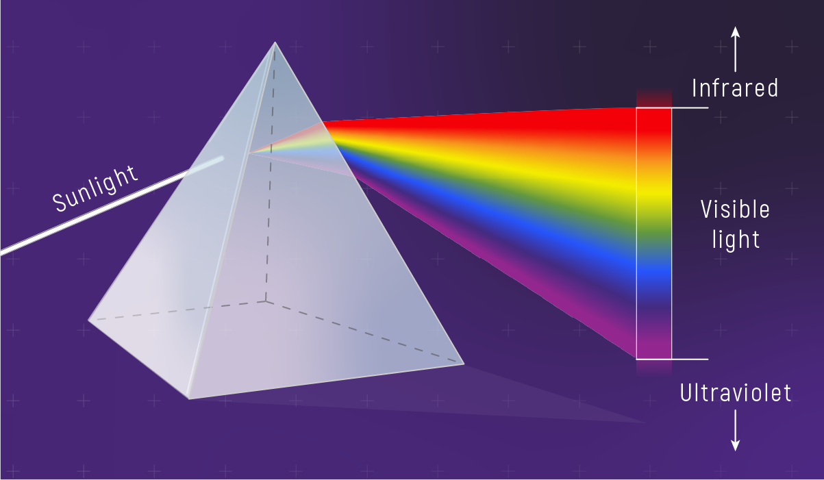
Figure 3:Dispersion Reveals Light’s Wavelength Components. A prism separates white sunlight into its constituent wavelengths through wavelength-dependent refraction. Visible spectrum spans 400-700 nm (violet to red), but sunlight also contains substantial UV (<400 nm) and infrared (>700 nm) invisible to our eyes. This dispersion principle underlies spectroscopy. (Credit: NASA/JWST)
1.1.2 The Fundamental Trinity: Speed, Wavelength, and Frequency
To decode the physics encoded in light, we need to understand the fundamental relationships governing electromagnetic radiation Let’s start with the relationship that governs all electromagnetic radiation:
where cm/s is the speed of light (in vacuum), is the wavelength (in cm), and is the frequency (in Hz or s). This isn’t just a formula to memorize – it’s telling us something important. The speed of light is constant in a vacuum, so wavelength and frequency are inversely proportional to one another – when one increases, the other must decrease. Long wavelengths mean low frequencies; short wavelengths mean high frequencies. This relationship is why we can use wavelength and frequency interchangeably when describing light.
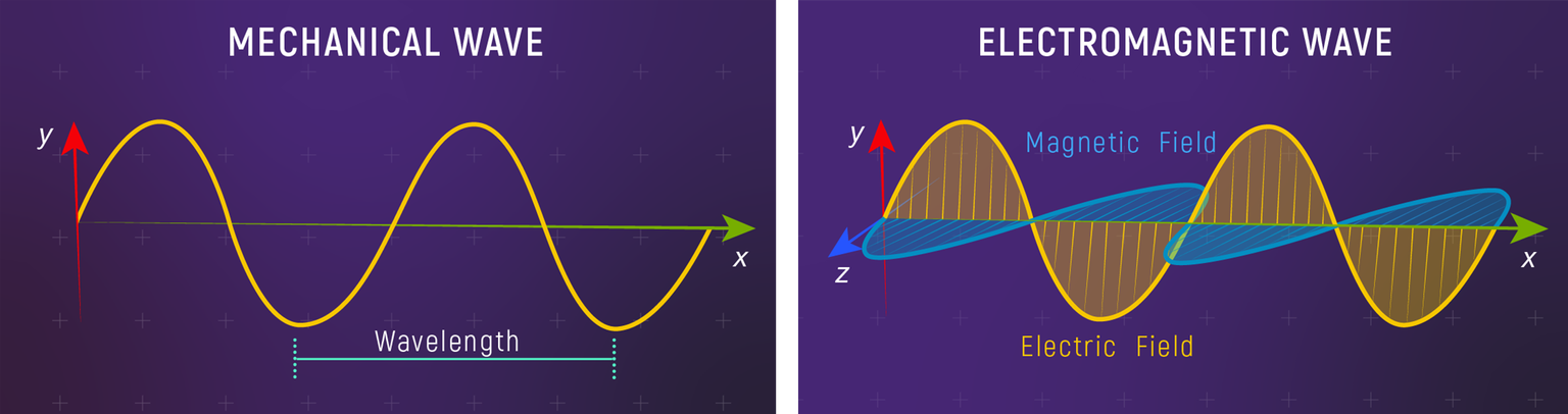
Figure 4:Electromagnetic vs Mechanical Waves. Left: Mechanical waves require matter to propagate—particles oscillate perpendicular to wave direction. Right: EM waves are self-propagating oscillations of perpendicular electric (yellow) and magnetic (blue) fields that travel at speed through vacuum. Wavelength determines the type of radiation while the field amplitudes determine intensity. (Credit: NASA/JWST)
But the real physics emerges when we include Planck’s revolutionary insight:
where erg·s is Planck’s constant, and is the photon energy in ergs. This equation is the Rosetta Stone of astronomy. It tells us that photon energy is directly proportional to frequency and inversely proportional to wavelength. High-energy phenomena produce high-energy photons with short wavelengths. Low-energy processes emit low-energy photons with long wavelengths.
1.1.3 The Electromagnetic Spectrum as a Physics Ladder
Now we can understand why different astronomical objects shine at different wavelengths. The electromagnetic spectrum isn’t just a list to memorize – it’s a ladder of physical processes, organized by energy.
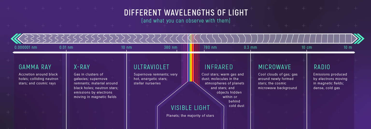
Figure 5:The Electromagnetic Spectrum as an Astrophysical Diagnostic Tool. Each wavelength band reveals different cosmic phenomena based on the physics of emission. Gamma rays probe particle acceleration in black holes and cosmic rays. X-rays trace million-degree gas in galaxy clusters and neutron stars. UV reveals hot stellar nurseries. Visible light shows stellar photospheres and planets. Infrared penetrates dust to reveal cool stars and molecular clouds. Microwaves trace cold gas and the CMB. Radio maps magnetic fields and dense molecular gas. (Credit: NASA/JWST)
Let’s work our way up this energy ladder, connecting each band to familiar astronomical phenomena:
Radio Waves and and Microwaves ( eV, cm) (1 eV-0.001 eV, 10 cm-1 mm)
What you know: Those gorgeous spiral arms in galaxy images, the 21-cm line of neutral hydrogen.
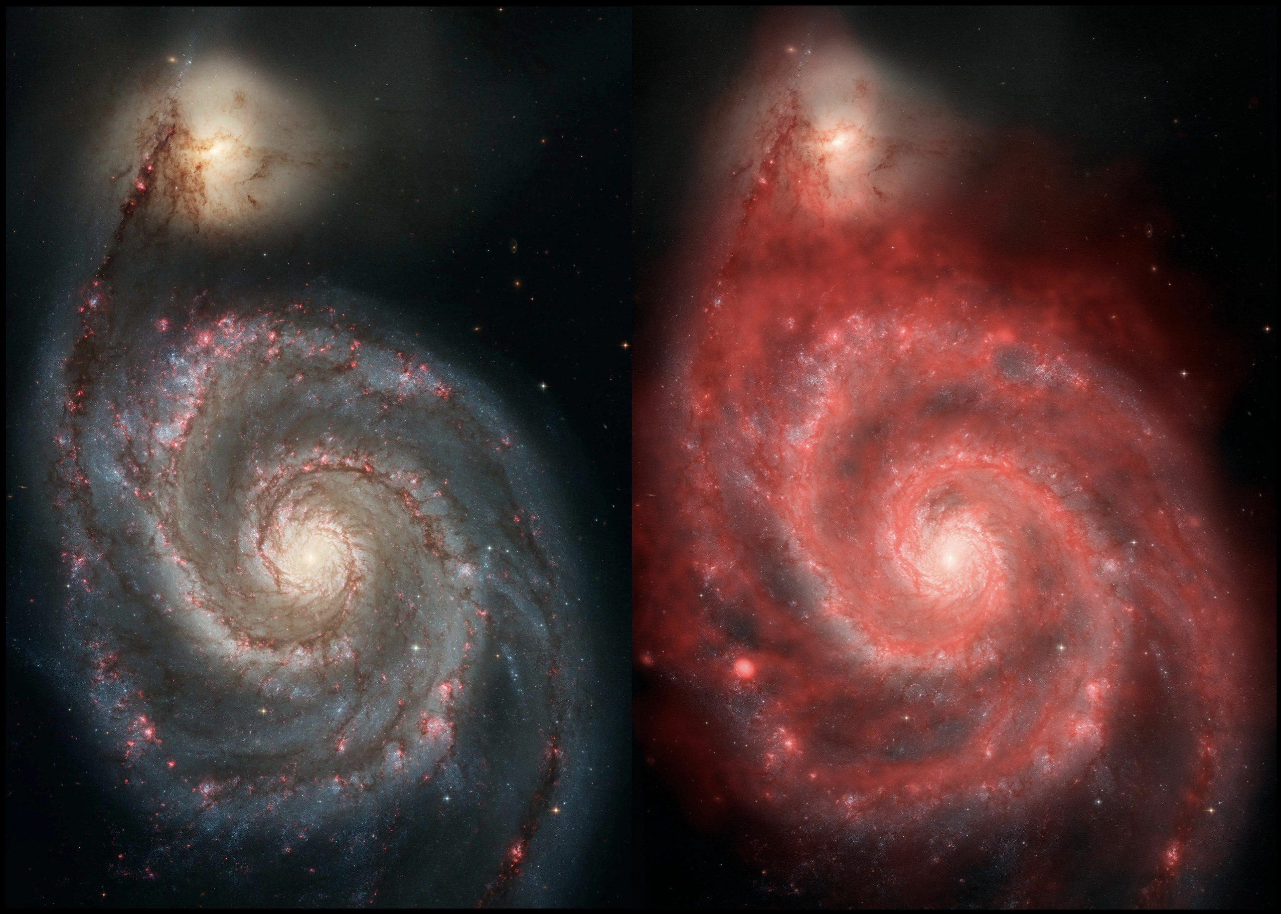
Figure 6:Same Galaxy, Different Physics: M51 Whirlpool Galaxy. Left: Optical (HST) shows billions of stars in spiral arms with dark dust lanes. Right: Radio (VLA 21-cm) reveals cold hydrogen gas (~100 K) extending farther than visible stars—the raw material for future star formation. Different wavelengths literally show different components: optical traces hot stars, radio traces cold gas reservoirs we’d otherwise miss entirely. (Credits: NASA/ESA/STScI/AURA; NRAO/AUI)
Starting our climb up the physics ladder: Cold gas clouds with temperatures of 10-100 K emit radio waves through magnetic field interactions and atomic spin flips. Radio photons carry the lowest energies on our ladder, revealing the coolest, most extended components of astronomical objects – the vast reservoirs of gas that will eventually form stars.
Infrared (IR) (0.001-1 eV, 1 μm-3 mm)
What you know: JWST’s ability to see through dust, thermal images of planets and cool stars.
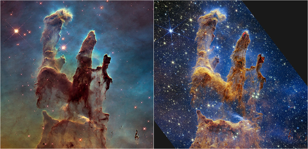
Figure 7:Infrared Reveals What Optical Cannot See: The Pillars of Creation. Left: Hubble’s optical view shows opaque dust pillars blocking background stars. Right: JWST’s near-infrared view penetrates the dust, revealing thousands of embedded stars and protostars (red points) invisible to Hubble. Infrared light passes through dust ~100× more easily than visible light because IR wavelengths are larger than typical dust grain sizes. (Credit: NASA, ESA, CSA, STScI)
Climbing higher on our physics ladder: Warm dust and molecules (100-1000 K) radiate thermal energy as infrared photons. This is the glow of stellar nurseries, planet-forming disks, and the dust grains themselves as they absorb starlight and re-radiate it at longer wavelengths. Wien’s law tells us exactly why: cooler objects peak at longer wavelengths.
Optical (Visible Light; 1-3 eV, 400-700 nm)
What you know: The colors we see with our eyes, stellar classifications, nebular emission lines.
Continuing our climb: Stellar photospheres (3000-50,000 K) and electronic transitions in atoms. The hydrogen-alpha line at 656 nm corresponds to exactly 1.89 eV – the energy difference between the second and third energy levels of hydrogen. Our eyes evolved to see this wavelength range precisely because our Sun emits most of its energy here.
Ultraviolet (UV) (3-100 eV, 10-400 nm)
What you know: Young, hot stars; regions of active star formation invisible to optical telescopes.
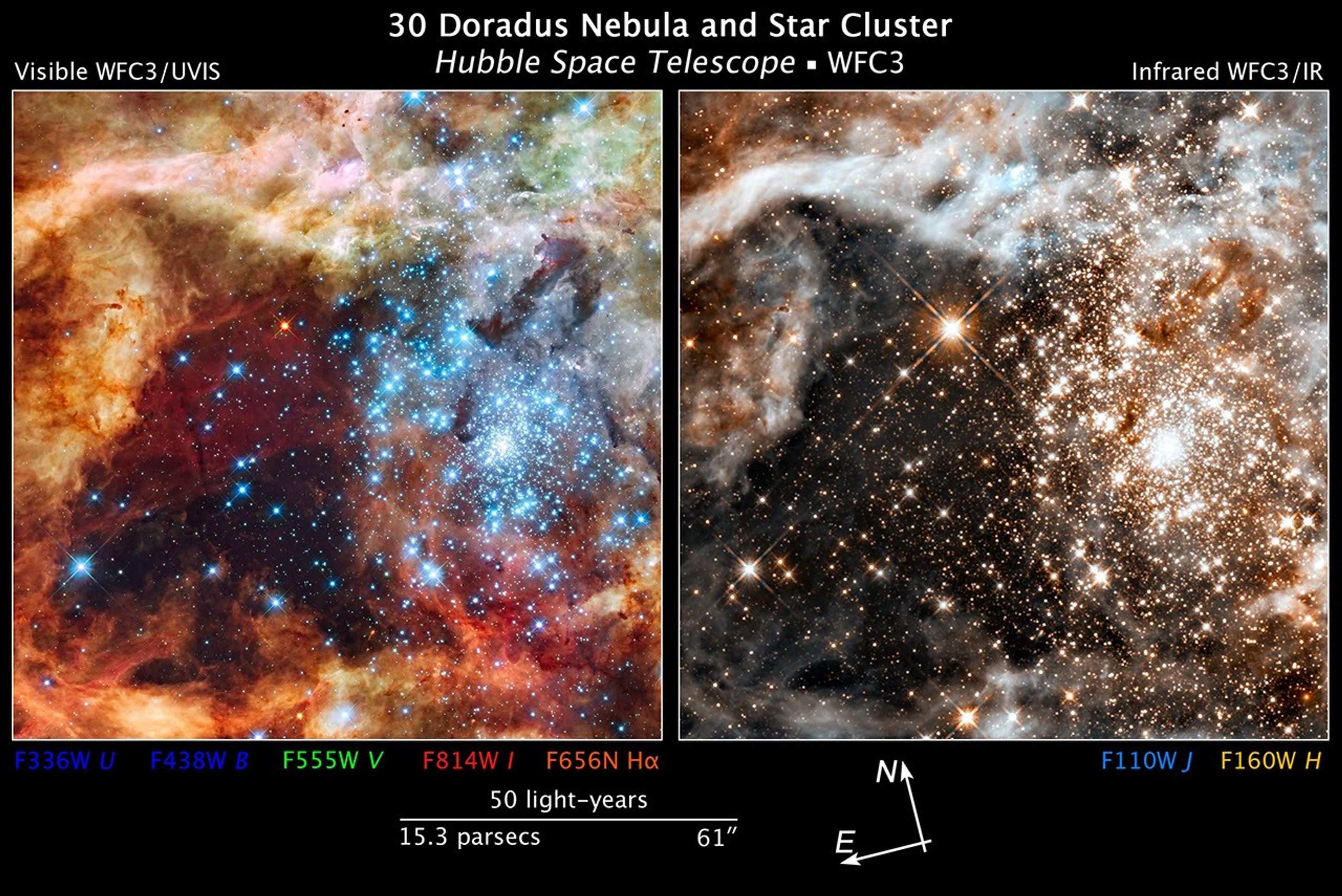
Figure 8:30 Doradus Star-Forming Region Across the Spectrum. This composite reveals how different wavelengths trace different temperatures and processes. Blue (UV) highlights the hottest, most massive stars (>30,000 K). Green/yellow (visible) shows intermediate-temperature stars and ionized gas. Red (near-IR) penetrates dust to reveal cooler, embedded stars and warm dust. The dark lanes that block visible light become transparent in infrared, demonstrating wavelength-dependent dust extinction. (Credit: NASA, ESA, F. Paresce, R. O’Connell, and the WFC3 Science Oversight Committee)
Higher up our physics ladder: Hot stellar atmospheres (>10,000 K) and high-energy atomic transitions. UV photons carry enough energy (>13.6 eV) to ionize hydrogen atoms, creating the glowing nebulae around massive stars. Only the most massive, shortest-lived stars produce significant UV radiation – making UV observations a direct tracer of recent star formation.
X-rays (100 eV-100 keV, 0.01-10 nm)
What you know: Accretion disks around black holes, supernova remnants, the hot gas between galaxies.
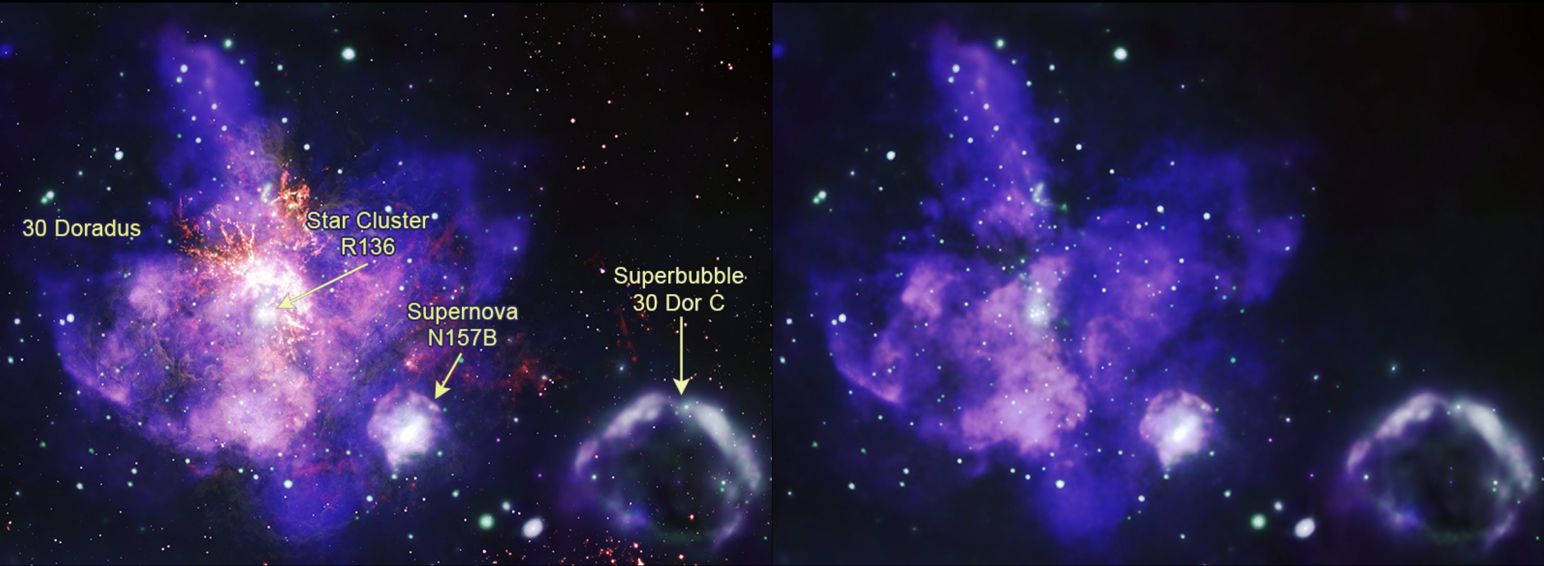
Figure 9:X-rays Reveal the Violent Heart of 30 Doradus. Left: Multi-wavelength composite showing the full star-forming complex. Right: Chandra X-ray view (blue) traces million-degree plasma carved out by shock-heated stellar winds and supernova explosions. These violent processes—invisible at other wavelengths—create bubbles and cavities of gas heated to millions of K. Only the most extreme astrophysical events produce X-ray photons (>100 eV), making this wavelength essential for understanding stellar feedback and energetics. (Credit: X-ray: NASA/CXC/PSU/L. Townsley et al.)
Climbing higher on our physics ladder: We’ve reached the realm of million-degree plasmas and violent shock heating. When stellar winds (≳1000 km/s) and supernova ejecta (~10,000 km/s) slam into the surrounding ISM, their enormous kinetic energy thermalizes—creating shock-heated gas at 10^7-10^8 K that then adiabatically expands and cools to ≳10^6 K, still hot enough to emit X-rays. In accretion disks around neutron stars and black holes, gravitational energy converts to heat just as efficiently. X-ray photons carry 100+ times more energy than visible light, revealing these violent processes that shape galaxies through stellar feedback.
Gamma Rays (>100 keV, <0.01 nm)
What you know: Supernova Remnants, Gamma-ray bursts, pulsars, cosmic ray interactions.
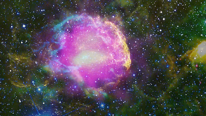
Figure 10:Gamma Rays Mark Cosmic Particle Accelerators: Supernova Remnant IC 443. Fermi gamma-ray emission (magenta) reveals where supernova shocks accelerate charged particles (electrons, protons, ions) to near light speed. When these cosmic rays collide with dense gas (cyan loops from WISE infrared), they produce gamma rays through pion decay—photons with energies >100 MeV that only arise from the universe’s most extreme particle acceleration. The infrared traces warm dust (blue to red: 3.4-22 μm), while optical (yellow) shows heated gas. Only gamma rays directly probe the cosmic ray acceleration that makes SNRs nature’s particle accelerators. (Credit: NASA/DOE/Fermi LAT Collaboration, NOAO, and WISE)
At the top of our physics ladder: Nuclear processes, matter-antimatter annihilation, and the most extreme magnetic fields. Gamma-ray photons carry so much energy that they can only be produced by the most violent events: stellar collapse, black hole mergers, or the decay of exotic particles. They’re the universe’s way of announcing its most dramatic moments.
The Pattern: As we move up the energy ladder, we’re probing increasingly violent and exotic physics:
Radio → Cold, extended gas reservoirs and magnetic fields
Infrared → Warm dust, stellar nurseries, and thermal processes
Optical → Stellar photospheres and ionized gas
UV → Hot stars and high-energy transitions
X-ray → Million-degree plasmas and violent processes
Gamma-ray → Nuclear furnaces and gravitational monsters
Each wavelength band reveals different components of the same astronomical objects.
1.1.4 Temperature’s Signature in Astrophysical Spectra
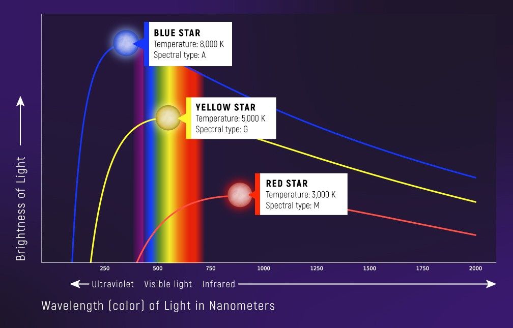
Figure 11:Wien’s Law in Action: Temperature Determines Peak Wavelength. Stars emit as nearly perfect blackbodies. Hotter stars emit more total energy and peak at shorter wavelengths. A blue star (8,000 K) peaks in UV/blue, Sun-like star (5,000 K) peaks in green/yellow, and cool red star (3,000 K) peaks in infrared. The peak wavelength follows Wien’s Law , allowing us to determine stellar temperatures from color alone. (Credit: NASA/JWST)
Wien’s displacement law connects an object’s temperature directly to its peak emission wavelength:
This isn’t an approximation – it’s exact physics emerging from Planck’s law, which describes the intensity of radiation emitted by a perfect blackbody at temperature across all wavelengths:
where erg/K is Boltzmann’s constant. The shape of this curve depends only on temperature, and its peak shifts to shorter wavelengths as temperature increases.
Wien’s law tells us that hotter objects emit more total energy and peak at shorter wavelengths. Cooler objects emit less energy and peak at longer wavelengths.
🟢 Example: Wien’s Law in Action
Let’s see what this tells us about familiar objects:
The Sun ( K):
This is green light! Our Sun peaks in the green, which is why human eyes evolved maximum sensitivity around 550 nm. We’re literally adapted to see our star’s peak output.
Red giant surface ( K):
This peaks in the near-infrared! Red giants appear red not just because they’re cool, but because their peak emission is beyond what our eyes can see.
Other key temperatures:
Warm dust in nebulae ( K): m (far-infrared)
Cosmic microwave background ( K): mm (microwave)
The key insight: When we observe an object’s spectrum and find its peak, we immediately know its temperature. But more profoundly, that temperature tells us what physical processes dominate. The spectrum reveals not just temperature but which physics matters – the dominant processes that shape what we observe.
This would be the end of the story if space were empty. But here’s where astronomy becomes truly challenging: the universe between us and every distant object is filled with gas and dust that fundamentally alters the light we receive. Understanding this transformation isn’t optional — it’s essential for interpreting any observation beyond our solar system. Not all photons emitted by distant objects reach our telescopes unchanged, and this intervening material leaves its own signature on the light...
🔧 Mathematical Toolkit for Part I
Fundamental Equations (CGS units throughout):
Wave equation:
cm/s (speed of light)
in cm (wavelength)
in Hz or s (frequency)
Photon energy:
erg·s (Planck’s constant)
in ergs (energy)
Wien’s law:
in K (temperature)
in cm (peak wavelength)
Extinction:
in erg cm s (flux)
in magnitudes (extinction)
Optical depth:
dimensionless (optical depth)
Key Conversions:
1 nm = 10-7 cm
1 μm = 10-4 cm
1 eV = erg
1 Å = 10-8 cm
Dimensional Analysis Check: Before calculating photon energy, let’s verify our units work out correctly:
The seconds cancel, the cm cancel, leaving us with energy in ergs as expected.
Sample Calculation - Green Light Photon Energy: For nm = cm:
Undefined control sequence: \cdotp at position 1: \̲c̲d̲o̲t̲p̲

E = \frac{hc}{\lambda} = \frac{(6.626 \times 10^{-27} \text{ erg·s}) \times (2.998 \times 10^{10} \text{ cm/s})}{5.5 \times 10^{-5} \text{ cm}} = 3.61 \times 10^{-12} \text{ erg} = 2.25 \text{ eV}
Notice that this 2.25 eV energy is typical for visible light—this isn’t coincidental, it matches the energy scale of outer electron transitions in atoms. The key insight: Photon energies and atomic physics are perfectly matched.
1.2 The Imperfect Journey: When Light Meets Matter
Priority: 🔴 Essential.
If space were truly empty, astronomy would be straightforward. A 30,000 K star would always appear brilliant blue-white, its spectrum perfectly encoding its surface conditions. We could determine distances from apparent brightness using the inverse square law, and stellar colors would directly reveal stellar temperatures. But space isn’t empty—between us and every celestial object lies the interstellar medium (ISM), a tenuous but crucial mix of gas and interstellar dust that fundamentally alters the light passing through it.
This isn’t a minor correction — it’s a complete transformation that can make a hot blue supergiant appear as cool and red as the Sun. Understanding this transformation isn’t optional; it’s essential for interpreting any astronomical observation beyond our solar system.
1.2.1 The Great Deception: When Hot Stars Masquerade as Cool Ones
Let’s start with a dramatic demonstration of dust’s transformative power. Consider a single B0V star — a stellar powerhouse with surface temperature 30,000 K that should appear blue-white in color. Let’s see what happens as we observe it through increasing amounts of interstellar dust.
📚 Stellar Spectral Types: The OBAFGKM Sequence
The Harvard Spectral Classification organizes stars by their photospheric temperature, revealed through their absorption line patterns. Originally alphabetical (A, B, C...), the sequence was reordered by temperature after physical understanding emerged.
The Modern Sequence (Hot → Cool):
| Class | Temperature | Color | Key Features | Example Stars |
|---|---|---|---|---|
| O | >30,000 K | Blue | Ionized He II lines, weak H | Alnitak (ζ Ori) |
| B | 10,000-30,000 K | Blue-white | Neutral He I, stronger H | Rigel, Spica |
| A | 7,500-10,000 K | White | Strongest H lines (Balmer) | Vega, Sirius |
| F | 6,000-7,500 K | Yellow-white | Weaker H, metals appear | Canopus, Procyon |
| G | 5,200-6,000 K | Yellow | Ca II H&K prominent | Sun, α Cen A |
| K | 3,700-5,200 K | Orange | Metals dominate, molecular bands | Arcturus, Aldebaran |
| M | 2,400-3,700 K | Red | TiO molecular bands | Betelgeuse, Proxima Cen |
Mnemonics: “Oh Be A Fine Girl/Guy, Kiss Me” (traditional) or “Only Bad Astronomers Forget Generally Known Mnemonics” (modern)
Luminosity Classes (added to letter):
I: Supergiants (Ia/Ib for bright/normal)
II: Bright giants
III: Giants
IV: Subgiants
V: Main sequence (dwarfs)
Example: The Sun is a G2V star (G-type, slightly hotter than mid-G, main sequence). Betelgeuse is M2Iab (cool red supergiant).
Physical Basis: Temperature determines which atoms/ions exist in the photosphere and which energy levels are populated, creating characteristic absorption patterns. Hot O-stars ionize hydrogen and helium. Cool M-stars allow molecules like TiO to form. The sequence represents a continuous temperature gradient, not discrete categories.
For this module: When we discuss extinction making a “B0V star appear like a K-star,” we mean its blue light (characteristic of 30,000 K) is so preferentially absorbed that its color mimics a 4,500 K star — a temperature error of 6×!
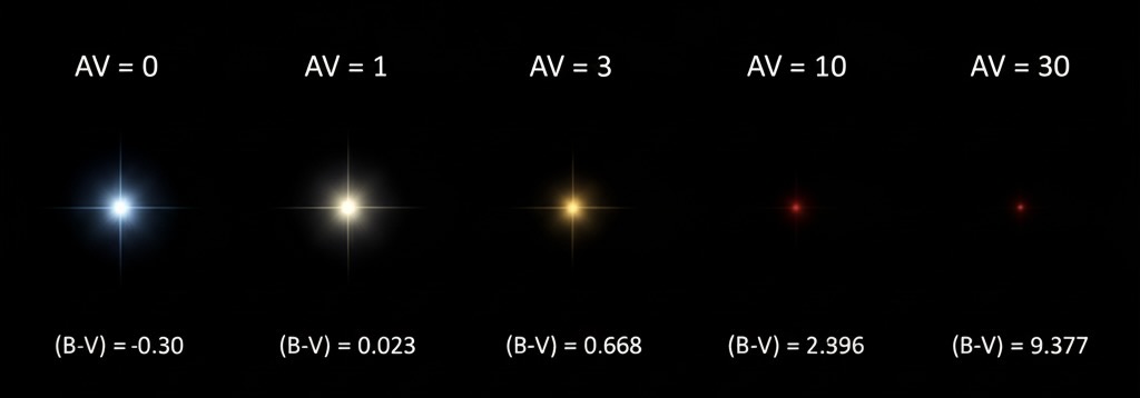
Figure 13:The Great Deception: How Dust Transforms Stellar Appearances. This sequence shows how a single B0V star ( K) would appear through progressively greater amounts of interstellar dust. Left: With no extinction (), the star appears as it truly is — brilliant blue-white with color index . Moving rightward: As extinction increases ( magnitudes), the star’s appearance transforms completely. By (common in the Galactic plane), it appears yellow like a Sun-like star. At (typical for star-forming regions), it looks like a cool red star with . By (toward the Galactic center), it vanishes entirely in optical light — a star that should be among the brightest in the sky simply disappears. This isn’t distance dimming — it’s wavelength-selective filtering that completely changes how we perceive stellar properties.
The transformation is startling:
No dust (): Brilliant blue-white, , blazing with the light of 40,000 Suns
Light dust (): Slightly dimmer and redder, but still recognizably a hot star
Moderate dust (): Now appears yellow-white like a Sun-like star,
Heavy dust (): Looks like a cool red giant,
Extreme dust (): Completely invisible in optical light
This isn’t science fiction — it’s the reality of Galactic astronomy. That “red giant” you observe might actually be a blue supergiant in disguise. The average extinction in the Galactic plane is about 1.8 magnitudes per kiloparsec in the V band. A star 10 kpc away experiences magnitudes of extinction—it appears 160 million times fainter than it actually is!
1.2.2 The Physics Behind the Transformation
When starlight encounters interstellar dust, two fundamental processes remove photons from our line of sight:
Absorption: The photon is captured and its energy converted to thermal energy, heating the dust grain. The grain then re-radiates this energy as thermal emission at far-infrared wavelengths—crucially, in random directions. The original photon heading toward us is gone, replaced by infrared photons scattered to the cosmic void.
Scattering: The photon interacts with electrons in the grain and is re-radiated in a different direction. The photon survives with its energy unchanged, but it’s no longer heading toward us. From our perspective, it might as well have been destroyed.
Both processes remove photons from the direct beam, creating extinction — the combined dimming effect that makes objects appear fainter than they actually are.
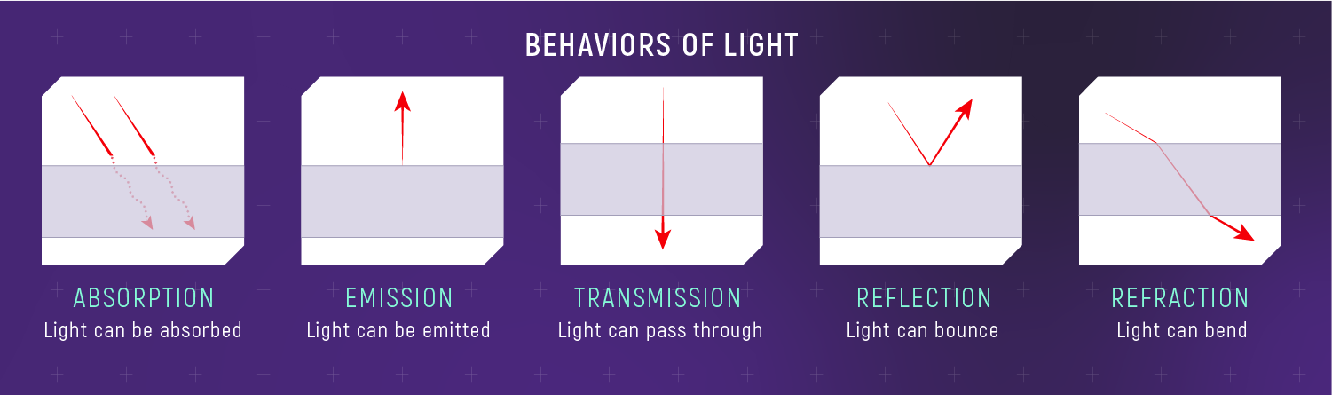
Figure 14:Fundamental Light-Matter Interactions for Radiative Transfer. Matter can absorb photons (converting energy to heat), emit photons (releasing energy), and reflect photons (redirecting without absorption). These three processes — quantified by the absorption per unit mass coefficient (opacity), emission coefficient , and albedo — form the basis of the radiative transfer equation. Different materials interact differently with different wavelengths. (Credit: NASA/JWST)
The key physics lies in how grain size relates to wavelength. Interstellar dust grains follow a size distribution roughly , where is the grain radius. This power law means smaller grains vastly outnumber larger ones. Most grains range from 0.005 to 1 μm, with a characteristic size around 0.1 μm that dominates optical scattering (cross-sectional area cm²). Notice that this 0.1 μm size is about one-fifth the wavelength of blue light—this size relationship is crucial for understanding why dust affects different colors differently.
When light wavelengths become comparable to grain size, we enter the Mie scattering regime where the interaction becomes most efficient. This size-wavelength relationship is the key to understanding why different colors of light interact differently with dust.
Here’s how this plays out for different wavelengths:
Blue light (450 nm) interacts strongly with abundant 0.1 μm grains
Red light (650 nm) interacts moderately with the same grains
Infrared light (2.2 μm) barely notices grains smaller than 1 μm
This creates wavelength-dependent extinction following approximately:
where for typical interstellar dust. Blue photons suffer much more extinction than red ones, creating the interstellar reddening effect — stars appear redder than their intrinsic colors because blue photons are preferentially removed from the beam.
1.2.3 Quantifying the Deception: The Mathematics of Correction
Here’s where astronomy becomes forensic science. Given what we observe, how do we determine what’s actually there? Let’s work through the standard procedure with a concrete example.
Example Calculation: Correcting for Extinction
Imagine you’re studying a star in our galaxy and want to determine its true distance and properties. You observe a star with:
Apparent V-band magnitude:
Observed color:
From its spectrum, you identify it as an A0V star, which should have:
Absolute magnitude:
Intrinsic color:
Step 1 - Calculate the color excess:
This measures how much redder the star appears than it should:
The star appears 1.5 magnitudes redder than it should—clear evidence of dust!
Step 2 - Connect reddening to total dimming:
Color excess tells us about the relative effect on different wavelengths, but we need the total dimming in the V-band to correct our distance. This requires understanding that the same dust causing reddening also causes overall dimming. The total-to-selective extinction ratio provides this crucial connection:
Step 3 - Determine total extinction:
For typical diffuse interstellar dust, . This ratio varies with environment:
Dense molecular clouds: (larger grains from coagulation)
Near hot stars: (smaller grains, large ones destroyed)
Galactic center: (harsh radiation environment)
Using the standard value:
Step 4: Correct the distance The true distance modulus accounts for extinction:
Converting to distance:
The consequence of ignoring dust: Without extinction correction, we would calculate:
We’d overestimate the distance by a factor of 8.5! This error cascades through everything:
Luminosity wrong by factor of
Stellar mass estimates completely off
Age determinations meaningless
Galaxy structure maps distorted
Physics isn’t optional in astronomy — it’s essential for getting the right answer.
The mathematical framework we’ve developed — color excess, extinction ratios, distance corrections — provides the foundation for correcting what we observe to reveal what’s actually there. But there’s an even more profound implication of wavelength-dependent extinction: it means the universe literally looks different when observed at different wavelengths. This isn’t just a pretty effect for making colorful images — it’s a fundamental tool for understanding astrophysical phenomena...
🧮 Quick Check 1.2
Test your understanding of extinction and reddening:
Warmup: If blue light is scattered more than red light by dust, what color will a dust cloud appear when illuminated by white light from behind? What about when viewed from the side?
Simple Calculation: A B5V star has intrinsic color . After passing through dust, you observe . What is the color excess ? If , what is ?
Conceptual Understanding: For mag toward a star-forming region, what fraction of V-band photons survive their journey? If infrared observations show , what fraction of K-band photons survive? Explain the dramatic difference.
Application: You want to study a young star cluster but can only see 50 stars in V-band due to dust extinction.
Before calculating: Do you expect to see more, fewer, or about the same number of stars in infrared K-band observations? Why?
Now calculate: Based on the infrared advantage, approximately how many cluster members might be detectable in K-band observations?
Click for Answers
Warmup: From behind, the cloud appears reddish (blue light removed, red transmitted). From the side, it appears bluish (scattered blue light reaches us, like Earth’s sky).
1. Color excess: magnitudes
Total extinction: magnitudes
2. V-band survival: (only 1 in 10,000 photons!)
K-band extinction: magnitudes
K-band survival:
The dramatic difference (factor of 3,600) occurs because K-band wavelength (2.2 μm) is much larger than typical grain sizes, so dust interaction is much weaker.
3. The brightness advantage in K-band is times brighter! If you can detect stars 100 times fainter (reasonable for modern IR detectors), you might see cluster members—revealing the cluster’s true population.
1.3 The Multi-Wavelength Universe: Many Faces of Reality
Different Wavelengths Reveal Different Physics in Sagittarius B2. This massive star-forming region located near the Galactic center (distance kpc) suffers extreme extinction ( reaching 50+ mag in dense regions), making it invisible in optical light. JWST’s MIRI (mid-infrared, 5-28 μm) detects thermal emission from warm dust (~100-300 K) heated by young stars, with only the hottest stars bright enough to shine through, while NIRCam (near-infrared, 0.6-5 μm) sees stellar photospheres and can penetrate dust to reveal thousands of stars. The dramatic difference occurs because MIR traces dust emission while NIR traces stellar emission, demonstrating why infrared observations are essential for understanding heavily obscured regions.
Priority: 🔴 Essential.
Here’s the revelation that transforms astronomy from pretty pictures to profound physics: the universe has many faces, and each wavelength shows us a different one. This isn’t poetic metaphor—it’s literal physical truth. When we observe an object like the Crab Nebula across the electromagnetic spectrum, we’re not seeing the same thing at different wavelengths; we’re seeing different physical components that happen to occupy the same space.
The Crab Nebula perfectly demonstrates this principle. The radio reveals relativistic electrons spiraling in magnetic fields, the optical shows ionized gas and stellar emission, the X-rays trace million-degree shocked plasma. Each wavelength is a window into different physics, and only by looking through all windows can we understand what we’re really seeing.
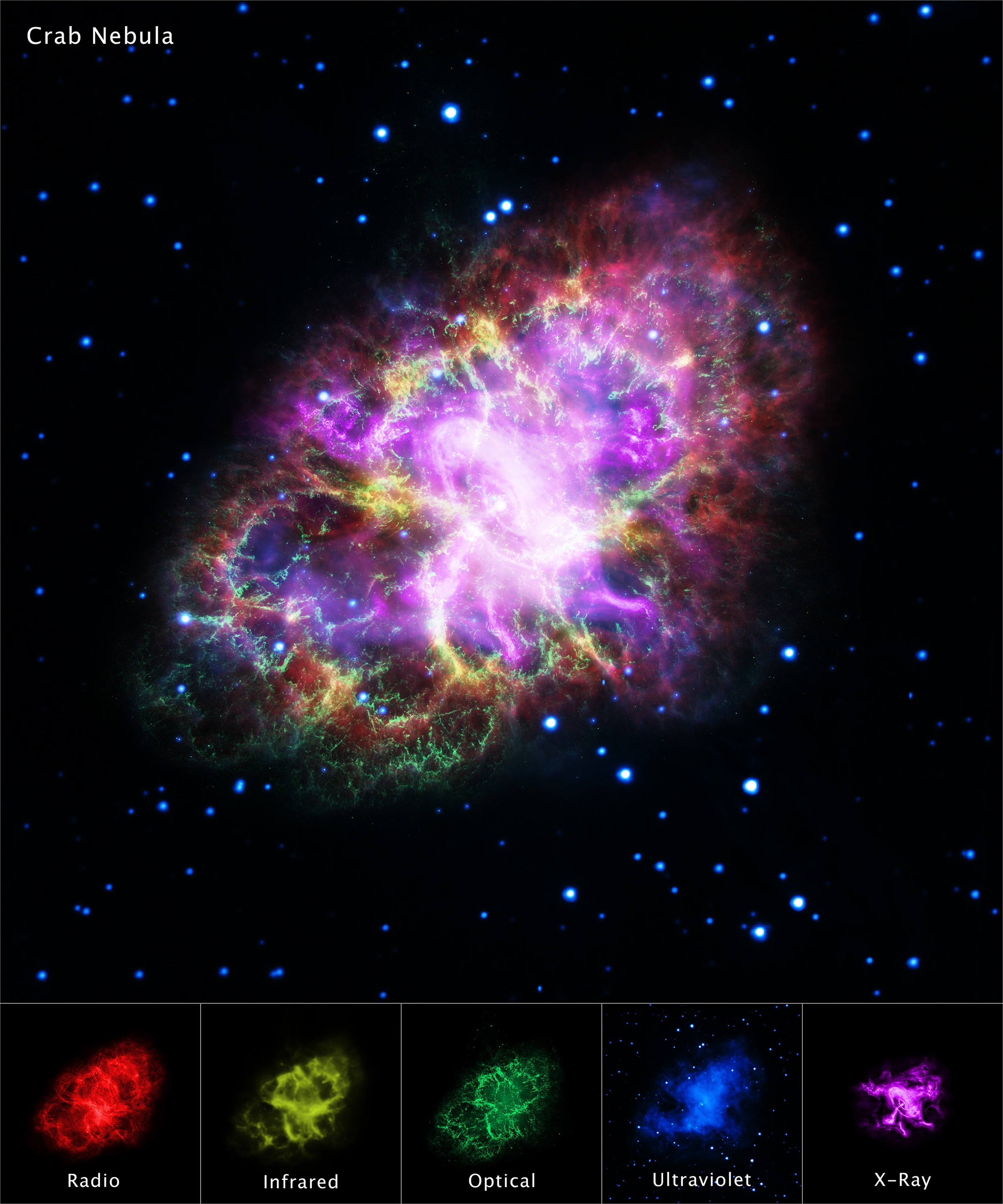
Figure 17:The Crab Nebula — A Cosmic Generator Revealed Across the Electromagnetic Spectrum. Top: This composite image combines data from five telescopes to show the 6,500 light-year distant remnant of a star that exploded in 1054 AD. The intricate structure results from the complex interplay between a pulsar spinning 30 times per second, its particle wind, and the supernova debris. Bottom row shows individual wavelength contributions: Radio (red, VLA): Synchrotron emission from relativistic electrons traces the full 11 light-year extent of magnetic fields permeating the nebula. Infrared (yellow, Spitzer): Warmer synchrotron emission mixed with thermal radiation from dust particles formed in the ejecta. Optical (green, Hubble): The iconic filamentary structure of ~10,000 K gas emitting hydrogen and oxygen spectral lines, sculpted by shocks and the pulsar wind. Ultraviolet (blue, XMM-Newton): The highest-energy synchrotron electrons and hottest gas reveal the most energetic non-thermal processes. X-ray (purple, Chandra): The dynamic pulsar wind nebula — a compact region where particles accelerated to near light-speed stream from the neutron star, creating structures invisible at other wavelengths. This “cosmic generator” at the nebula’s heart produces energy at the rate of 1,000 Suns. Each wavelength reveals different particles, temperatures, and physical processes occurring simultaneously in the same cosmic explosion remnant. Credits: NASA/CXC/SAO. Learn more about this multi-wavelength observation.
1.3.1 Same Object, Different Physics: The Crab Nebula Revealed
Let’s examine the Crab Nebula—the remnant of a star that exploded in 1054 AD—across the electromagnetic spectrum to see how different wavelengths reveal different physics:
Radio (GHz to MHz frequencies, meter to cm wavelengths): We see synchrotron emission from electrons with Lorentz factors spiraling in ~100 μG magnetic fields. The emission traces the full extent of the nebula—about 11 light-years across. The radio spectral index (where ) tells us the electron energy distribution.
Physics revealed: Magnetic field structure, particle acceleration efficiency, total energy in relativistic particles.
Infrared (1-100 μm, 0.01-1 eV): Two components appear: synchrotron from lower-energy electrons and thermal emission from ~40 K dust formed in the supernova ejecta. About 0.1 of dust—a significant fraction of the ISM’s dust budget comes from supernovae.
Physics revealed: Dust formation in extreme environments, continuation of the synchrotron spectrum.
Optical (400-700 nm, 2-3 eV): Beautiful filamentary structure appears—dense knots of gas at ~10,000 K emitting hydrogen Balmer lines, [O III], and other forbidden transitions. The famous blue-white glow comes from synchrotron emission from electrons with .
Physics revealed: Gas temperature and density, elemental abundances, highest-energy electrons.
X-ray (0.1-10 keV): A completely different structure emerges — a ring with jet-like features powered by the pulsar wind. The torus and jets show particles accelerated to (relativistic Lorentz factor). The pulsar itself pulses 30 times per second in X-rays.
Physics revealed: Pulsar wind termination shock, particle acceleration to extreme energies, magnetic reconnection sites.
Gamma-ray ( MeV): Only the pulsar is visible — a lighthouse beaming gamma rays as it spins. Pulsed emission up to GeV energies requires particles accelerated in the pulsar magnetosphere to Lorentz factors .
Physics revealed: Extreme particle acceleration, pulsar emission mechanisms, potential for producing cosmic rays (relativistic charged particles).
Each wavelength isn’t just providing a different view — it’s revealing different physical components and processes. Without radio, we’d miss the magnetic field structure. Without X-rays, the pulsar wind would be invisible. Without optical, we wouldn’t know the gas composition. The complete picture requires the complete spectrum.
Multi-Wavelength Synthesis: The Whole is Greater Than the Parts
Here’s the crucial insight that elevates observational astronomy to quantitative astrophysics: combining wavelengths reveals the physical mechanisms driving what we observe, not just what things look like. Multi-wavelength synthesis transforms catalogs of objects into maps of physical processes — and crucially, lets us test whether our theories match reality. When radio reveals magnetic fields, X-rays trace shocks, and optical shows ionized gas all in the predicted locations with the right energies, we know our models likely work. Consider determining the 3D structure and dynamics of the Crab’s pulsar wind nebula — impossible from any single wavelength:
Radio polarization observations → Magnetic field direction and strength throughout the nebula
Optical proper motion measurements → Expansion velocity vectors (1,500 km/s radially)
X-ray morphology and spectroscopy → Shock front locations and particle acceleration sites
Combined 3D analysis → Complete reconstruction of the relativistic flow pattern
Only by synthesizing all three can we map how the pulsar injects 1038 erg/s into the surrounding medium, creating the complex torus-and-jet structure visible in X-rays. This synthesis reveals the pulsar wind’s 3D dynamics and energy transport mechanisms—physics no single wavelength could demonstrate.
The power of multi-wavelength synthesis transforms astronomy from “collecting pretty pictures” to “reconstructing 3D astrophysical processes.”
This qualitative understanding of different physics becomes even more powerful when we make it quantitative.
The Transparency Revolution: Quantifying Wavelength Advantage
The power of multi-wavelength astronomy becomes quantitative when we consider how dust transparency changes with wavelength. As we saw in Section 1.2, the extinction follows , creating dramatic differences in transparency.
🔗 Example: NGC 3603 Through Multiple Eyes
Let’s apply this transparency revolution to our threading example NGC 3603 with its mag of dust:
Optical (V-band, 551 nm):
Extinction: mag
Transmission: (only 1% of light gets through!)
We see: ~100 brightest blue supergiants, miss most of the cluster
Near-IR (K-band, 2.17 μm):
Extinction: mag
Transmission: (42% gets through)
We see: >10,000 stars including solar-mass members
Mid-IR (10 μm):
Extinction: mag
Transmission: (91% gets through!)
We see essentially the complete cluster plus embedded protostars.
The 91× transparency gain from V to 10 μm transforms NGC 3603 from a sparse group of blue stars into one of the Milky Way’s most massive young clusters!
Your Learning Transformation: From Pictures to Physics
Take a moment to recognize how dramatically your perception has evolved through this module. When you started Section 1.1, an astronomical image was simply a beautiful picture. Now you see something fundamentally different:
What you now see in every astronomical image:
Red nebular glow → Hydrogen recombination at precisely 656.3 nm, revealing 10,000 K ionized gas
Dark dust lanes → 0.1 μm grains creating wavelength-dependent extinction following
Blue star-forming regions → 35+ eV photons ionizing oxygen, tracing massive stars >30
Multi-wavelength composites → Different physical components occupying the same space
You’ve developed the professional astronomer’s eye — the ability to decode quantitative physics from photons. This transformation from aesthetic appreciation to physical understanding is the essence of scientific literacy.
The deeper insight: Every wavelength tells a physics story. Every color encodes temperature, density, and composition. Every shadow reveals dust properties. The universe’s first galaxies, exoplanet atmospheres, and stellar nurseries all reveal their secrets through the same wavelength-dependent physics you’ve just conquered.
- Zhang, X., & Green, G. M. (2025). Three-dimensional maps of the interstellar dust extinction curve within the Milky Way galaxy. Science, 387(6739), 1209–1214. 10.1126/science.ado9787