Part 2: From Beliefs to Mathematics
How We Formalize Intuition into Rigorous Inference | Inferential Thinking Module 5 | ASTR 596
Learning Outcomes
By the end of Part 2, you will be able to:
Explain why probability is the unique extension of logic to uncertainty using Cox’s theorems
Distinguish between likelihood P(data|parameters) and posterior P(parameters|data)
Construct likelihood functions from physics models and measurement uncertainties
Transform astronomical knowledge into mathematical prior distributions
Derive Bayes’ theorem from first principles using counting arguments
Apply the complete Bayesian framework to Cepheid distance measurement
Connect each component to concepts from the Statistical Thinking module
Part 2: From Beliefs to Mathematics
How do we transform vague beliefs into rigorous inference?
Core Question: How do we transform statements like “this star probably has little dust” into mathematical frameworks that can process data and quantify uncertainty?
2.1 Probability as Extended Logic
Priority - 🔴 Essential:
The Limits of True and False
Classical logic, the foundation of mathematics since Aristotle, deals in absolutes. A statement is either true or false. A star either has dust extinction or it doesn’t. But astronomy doesn’t work this way. When we observe a reddened star, we can’t say with certainty “this star is behind dust.” The reddening could be intrinsic (the star is cool), it could be from dust, it could be from measurement error, or some combination. We need a framework that handles degrees of belief.
Consider the logical chain an astronomer faces:
If a star is behind dust, it will appear reddened (TRUE)
This star appears reddened (TRUE)
Therefore... what?
Classical logic fails us here. The star MIGHT be behind dust, but it might also be intrinsically red. We need to say something like “the reddening increases the plausibility that the star is behind dust, but doesn’t prove it.” This is where probability enters — not as a choice, but as a necessity.
Probability: The Language of Plausible Reasoning
In the 1940s, physicist Richard Cox asked a profound question: If we want to extend logical reasoning to handle uncertainty, what rules must we follow? His answer was stunning — there is only ONE consistent way to reason with uncertainty, and it’s probability theory.
Cox started with desiderata (requirements) that any system of plausible reasoning should satisfy:
Degrees of Plausibility: Propositions have degrees of plausibility, represented by real numbers
Consistency: If a conclusion can be reached in multiple ways, all ways must give the same answer
Correspondence: In the limit of certainty, plausible reasoning must reduce to deductive logic
Universality: The system should handle any proposition we can state
From just these requirements — which seem almost too basic to be powerful — Cox proved that plausible reasoning MUST follow the rules of probability theory. Not “should” or “could”—MUST.
From Astronomical Intuition to Mathematical Probability
Astronomers have always thought probabilistically, even before formalizing it. When Henrietta Leavitt said “these stars are probably at the same distance,” she was expressing a degree of belief. When modern astronomers say “this galaxy probably contains dark matter,” they’re doing plausible reasoning. Probability theory just makes this reasoning mathematically rigorous.
Let’s see how astronomical statements become probabilities:
Qualitative Statement → Probability Statement
“This star is probably nearby” → P(d < 100 pc) = 0.8
“Little dust in this direction” → P(A_V < 0.1 mag) = 0.9
“Cepheid follows the P-L relation” → P(|ΔM| < 0.15) = 0.68
Each transformation takes vague intuition and makes it precise. The numbers aren’t arbitrary—they encode our accumulated knowledge from centuries of observations.
The Cepheid Example: From Logic to Probability
Let’s apply this to our running Cepheid example. Using classical logic:
What we know for certain:
The star’s brightness varies periodically (TRUE)
The period is 5.366 days (TRUE)
Longer-period Cepheids are intrinsically brighter (TRUE from P-L relation)
What we can’t deduce with certainty:
The star’s distance (depends on intrinsic brightness)
The amount of dust extinction (degenerate with distance)
Whether it follows the standard P-L relation (metallicity effects?)
Enter probability:
[needs Bayes!]
Probability extends our logical reasoning to handle these uncertainties systematically.
Why Not Other Systems?
You might wonder: Why probability? Couldn’t we use fuzzy logic, possibility theory, or some other framework? Cox’s theorems say no—if we want consistency, we’re forced to use probability.
Here’s what happens with alternatives:
Fuzzy Logic: Handles vagueness (“very hot star”) but not uncertainty about facts Interval Arithmetic: Gives ranges but loses information about likelihood within the range Possibility Theory: Lacks the mathematical structure needed for updating with evidence
Only probability theory provides:
Consistent updating with new information (Bayes’ theorem)
Proper handling of correlations between variables
Natural incorporation of measurement uncertainties
Recovery of deductive logic in the limit of certainty
This uniqueness is profound. It means that aliens doing astronomy would use the same probability theory we do—not because they learned it from us, but because mathematics forces it upon any consistent reasoner.
2.2 Likelihood: Encoding Physics as Probability
Priority: 🔴 Essential
The Direction That Physics Gives Us
Physics naturally runs forward—from causes to effects, from parameters to observations. If we know a star’s temperature, we can predict its spectrum. If we know a Cepheid’s period and intrinsic brightness, we can predict its apparent magnitude at any distance. This forward direction is what physics provides, and it’s encoded in the likelihood function.
But here’s the critical insight that confuses many: The likelihood is NOT the probability of the parameters. It’s the probability of the data given the parameters. This distinction is subtle but fundamental.
Consider measuring a Cepheid’s brightness:
Forward (Physics): Given M = -3.5, d = 2.5 Mpc → predict m = 21.5
Inverse (Inference): Given m = 21.5 ± 0.1, P = 5.4 days → infer d = ?
The likelihood handles the forward direction. It says: “If the distance were 2.5 Mpc, how probable is it that we’d measure m = 21.5?” This is fundamentally different from asking “Given we measured m = 21.5, what’s the probability the distance is 2.5 Mpc?”
Building a Likelihood from Physics
Let’s construct a real likelihood function for our Cepheid. We start with the physics—the Period-Luminosity relation discovered by Leavitt:
The Physics Model:
where M_V is absolute V-band magnitude and P is period in days.
Adding Distance: The distance modulus relation connects intrinsic and apparent brightness:
where d is distance in parsecs.
Combining the Physics:
This is our deterministic model—given P and d, we predict m. But observations aren’t perfect...
From Deterministic Model to Probabilistic Likelihood
Real measurements have uncertainties. Our CCD has read noise, the atmosphere scintillates, and Cepheids have intrinsic scatter in their P-L relation. We need to transform our deterministic model into a probability distribution.
Step 1: Identify the uncertainties
Measurement error: σ_m ≈ 0.05 mag (photon noise + systematics)
Intrinsic scatter: σ_int ≈ 0.15 mag (Cepheids aren’t perfect standard candles)
Total uncertainty: σ_total = √(σ_m² + σ_int²) ≈ 0.16 mag
Step 2: Choose a noise model From the Statistical Thinking module, we learned about the Central Limit Theorem—many small random effects sum to a Gaussian distribution. Both measurement errors and intrinsic scatter arise from many small effects, so we use a Gaussian noise model.
Step 3: Write the likelihood
where we’ve added extinction A_V to our model (making it more realistic).
The Likelihood in Practice
def cepheid_likelihood(params, observations):
    """
    Likelihood for Cepheid distance measurement.

    Physics model + measurement uncertainty = likelihood
    """
    distance, extinction = params  # What we want to infer
    period, apparent_mag, mag_error = observations  # What we measured

    # Physics: Period-Luminosity relation (Leavitt Law)
    absolute_mag = -2.43 * (np.log10(period) - 1) - 4.05

    # Physics: Distance modulus
    distance_modulus = 5 * np.log10(distance) - 5

    # Physics: Extinction dims the star
    predicted_mag = absolute_mag + distance_modulus + extinction

    # Statistics: Gaussian noise model
    intrinsic_scatter = 0.15  # Cepheids aren't perfect standard candles
    total_sigma = np.sqrt(mag_error**2 + intrinsic_scatter**2)

    # The likelihood: How probable is our observation given these parameters?
    residual = apparent_mag - predicted_mag
    log_likelihood = -0.5 * (residual/total_sigma)**2 - np.log(total_sigma * np.sqrt(2*np.pi))

    return np.exp(log_likelihood)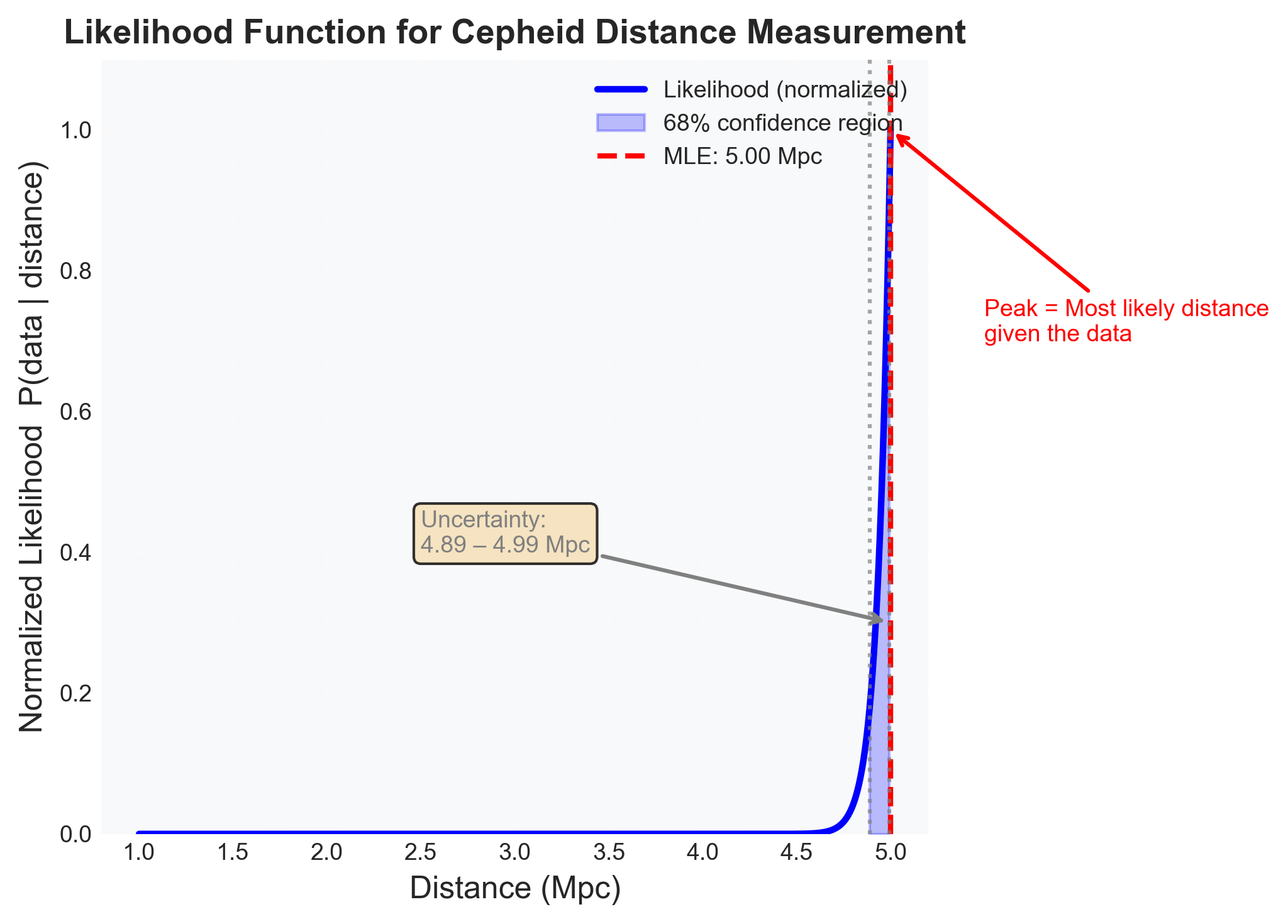
Figure 1:Likelihood function for Cepheid distance measurement. This figure shows how the likelihood P(data|distance) quantifies the compatibility between our observations and different distance hypotheses. The normalized likelihood (peak = 1.0) peaks at the maximum likelihood estimate (MLE) of d ≈ 5.00 Mpc, representing the distance most consistent with the observed apparent magnitude m = 25.3 ± 0.05 mag and period P = 10 days. The shaded 68% confidence region (blue) indicates the range of distances that are reasonably compatible with the data, spanning approximately 4.89–4.99 Mpc. The narrow width of this likelihood demonstrates high constraining power—the precise photometry and well-calibrated P-L relation provide strong constraints on distance. Note that this is NOT the probability of the distance being correct (that requires the posterior), but rather how probable our observation would be if the distance were at each value. The sharp rise near the peak shows that small changes in distance cause large changes in the predicted magnitude, making the data highly informative about distance.
Common Likelihood Pitfalls
Pitfall 1: Forgetting intrinsic scatter If you only include measurement error, you’ll be overconfident. Real astronomical objects have intrinsic variation that must be included in the likelihood.
Pitfall 2: Assuming Gaussian errors From Statistical Thinking, we know the CLT gives us Gaussians for many small effects. But what about outliers? Cosmic rays? Variable stars misclassified as Cepheids? Real data often has heavy tails, requiring robust likelihoods (like Student-t distributions).
Pitfall 3: Ignoring correlations If you observe multiple Cepheids with the same telescope, their measurements share systematic errors. The likelihood needs the full covariance matrix, not just individual error bars.
Pitfall 4: Confusing likelihood with posterior Remember: Likelihood is P(data|parameters), NOT P(parameters|data). Mixing these up leads to incorrect inferences.
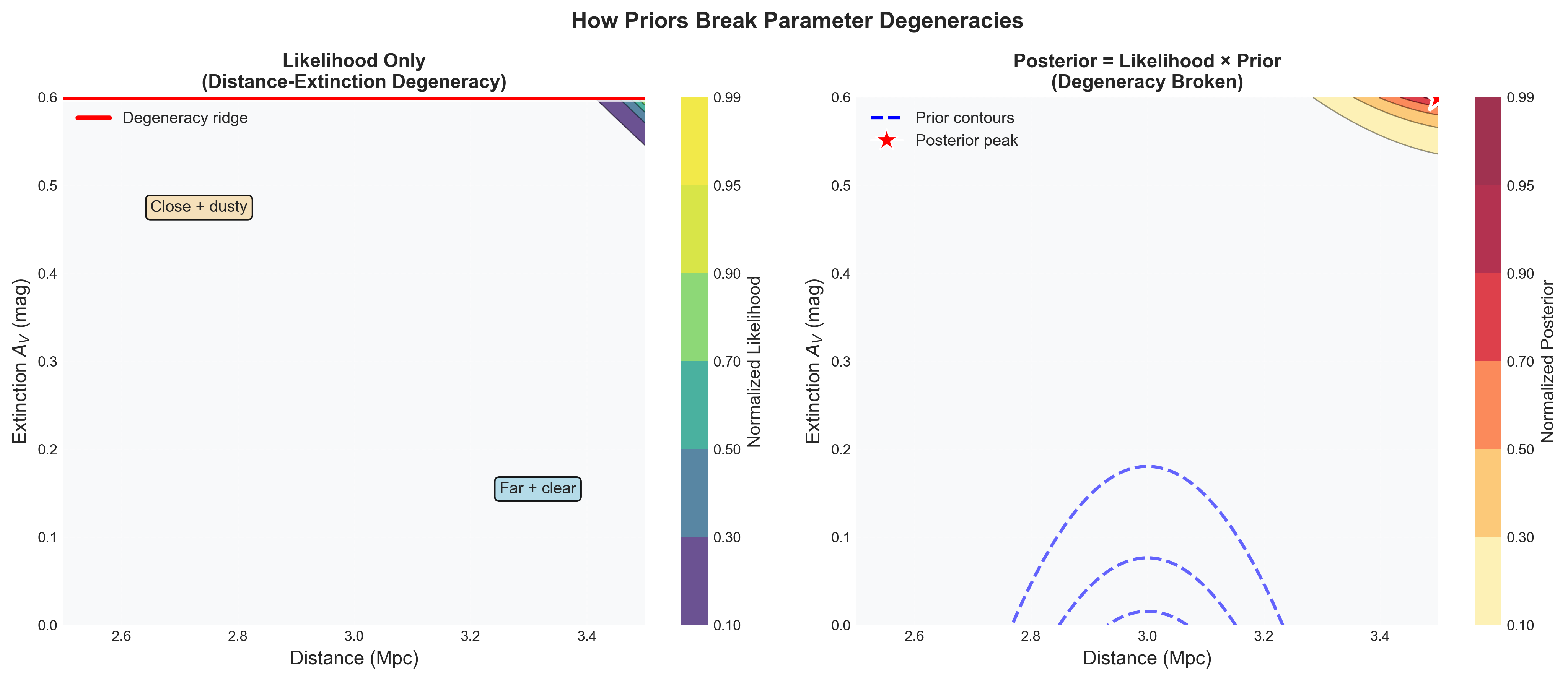
Figure 2:How priors break parameter degeneracies in 2D likelihood spaces. This side-by-side comparison demonstrates a fundamental challenge in astronomical inference: parameter degeneracy. Left panel (Likelihood Only): The distance-extinction degeneracy ridge (red line) shows that many parameter combinations produce equally good fits to the data. A star could be close and dusty (d ≈ 2.6 Mpc, A_V ≈ 0.5 mag) OR far and clear (d ≈ 3.4 Mpc, A_V ≈ 0.1 mag)—both predict the same observed magnitude. The likelihood alone cannot distinguish these scenarios because dust extinction and distance have similar effects on apparent brightness. Right panel (Posterior with Prior): Adding physically motivated priors breaks this degeneracy. A Gaussian prior on distance (from previous LMC measurements: 3.0 ± 0.15 Mpc, shown as blue dashed contours) combined with an exponential prior on extinction (most sightlines have low A_V, based on dust maps) concentrates probability mass on a single solution (red star). The posterior now strongly favors d ≈ 3.0 Mpc with A_V ≈ 0.2 mag. Key pedagogical insight: Priors aren’t subjective opinions—they encode objective astronomical knowledge (previous measurements, dust distribution statistics) that resolves ambiguities the data alone cannot. This is how the cosmic distance ladder works: each rung’s posterior becomes the next rung’s prior, progressively breaking degeneracies from local to cosmological scales.
The Deep Connection to Information Theory
The likelihood encodes information about parameters contained in the data. In information theory terms, it quantifies how “surprised” we should be by the observations given different parameter values. High likelihood = unsurprising (expected given the parameters). Low likelihood = surprising (unexpected given the parameters).
The width of the likelihood function tells us about information content:
Narrow likelihood: Data strongly constrains parameters (high information)
Broad likelihood: Data weakly constrains parameters (low information)
Flat likelihood: Data provides no constraint (zero information)
For our Cepheid, a precise brightness measurement gives a narrow likelihood in distance. A noisy measurement gives a broad likelihood. This width—the Fisher information—fundamentally limits how well we can measure distance regardless of our analysis method.
Connection to Statistical Thinking
Remember from the Statistical Thinking module that temperature is the width of the velocity distribution? The likelihood plays a similar role—it encodes the “width” of possible observations given parameters. Just as temperature describes the spread in molecular velocities, the likelihood describes the spread in possible observations.
The Central Limit Theorem from Statistical Thinking justifies our Gaussian likelihoods. When many small effects contribute to measurement error, their sum approaches a Gaussian. This is why Gaussian likelihoods are ubiquitous in astronomy—not by choice, but by mathematical necessity.
2.3 Priors: Quantifying What We Already Know
Priority: 🔴 Essential
The Knowledge We Bring to Every Observation
No observation is interpreted in a vacuum. When Henrietta Leavitt observed Cepheids in the Small Magellanic Cloud, she brought the belief that these stars were roughly equidistant. When Edwin Hubble used Cepheids to measure the distance to Andromeda, he brought Leavitt’s P-L calibration. Every measurement builds on previous knowledge—this is what priors formalize.
Consider what you implicitly know before observing tonight’s Cepheid:
Distances are positive (d > 0)
It’s probably in our galaxy (d < 30 kpc) or a nearby galaxy (d < 10 Mpc)
Extinction only reddens, never bluens (A_V ≥ 0)
Most sightlines have modest extinction (A_V < 2 mag)
The P-L relation has limited scatter (σ ≈ 0.15 mag)
This isn’t subjective opinion—it’s accumulated astronomical knowledge from centuries of observations. Priors transform this knowledge into mathematical form.
Types of Priors in Astronomy
Physical Constraint Priors These encode fundamental physical limits:
def distance_prior(d):
    """Distance must be positive"""
    return 1.0 if d > 0 else 0.0

def extinction_prior(A_V):
    """Extinction can only redden light"""
    return 1.0 if A_V >= 0 else 0.0

def mass_prior(M):
    """Stars have limited mass range"""
    if 0.08 < M < 150:  # Solar masses
        return 1.0
    else:
        return 0.0
Population Priors These encode knowledge about astronomical populations:
The Initial Mass Function (IMF) tells us most stars are low-mass:
The galactic extinction distribution from dust maps:
The period distribution of Cepheids:
Hierarchical Priors These capture how individual objects relate to populations:
# Individual Cepheid draws from population
population_mean_M = -2.43 * (log_P - 1) - 4.05
population_scatter = 0.15
individual_M ~ Normal(population_mean_M, population_scatter)

# Population parameters themselves have priors
population_scatter ~ HalfNormal(0.2)  # Must be positive, probably small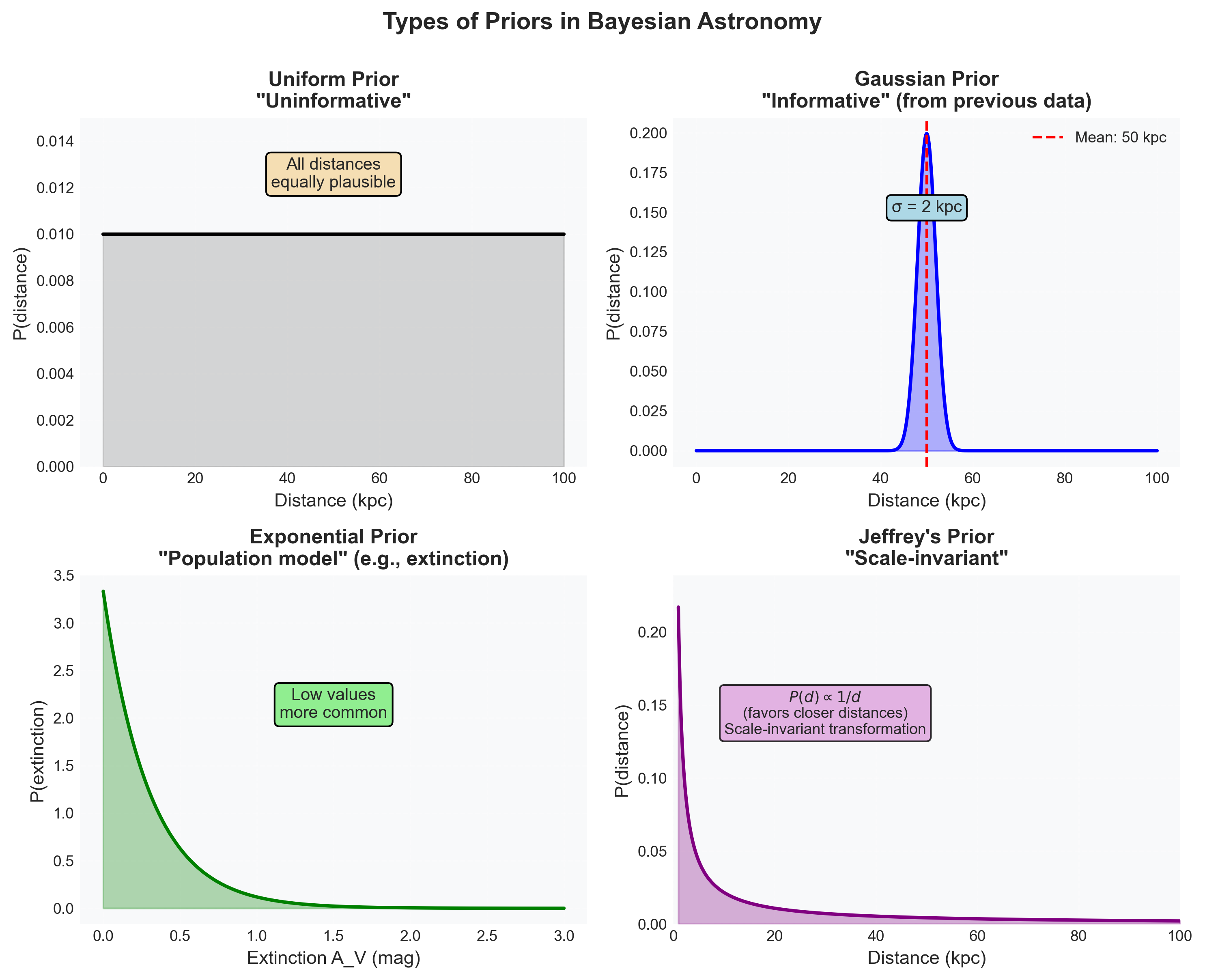
Figure 3:Four fundamental types of priors in Bayesian astronomy. This figure illustrates how different types of prior knowledge are mathematically encoded. Top-left (Uniform Prior): Represents maximum ignorance—all distances from 0 to 100 kpc are equally plausible. While called “uninformative,” it actually encodes strong assumptions (e.g., linear scale is appropriate) and is never truly objective. Used when we genuinely lack information or want to let data dominate. Top-right (Gaussian Prior): Encodes previous measurements—here, a galaxy distance of 50 ± 2 kpc from earlier studies. This “informative” prior concentrates probability where observations have constrained parameters. Essential for hierarchical inference (cosmic distance ladder). Bottom-left (Exponential Prior): Represents population models—extinction follows an exponential distribution because most sightlines have low dust column density, with progressively fewer having high extinction. Based on empirical regularities from dust maps and galactic structure. The scale parameter (here 0.3 mag) comes from astronomical data, not guesses. Bottom-right (Jeffrey’s Prior): A scale-invariant prior P(d) ∝ 1/d that treats all scales equally—doubling from 1→2 kpc is as significant as 50→100 kpc. Derived from information theory to be maximally non-informative with respect to parameter transformations. Used when we want to encode complete ignorance about a scale parameter. Critical insight: Each prior type serves a specific purpose and encodes objective astronomical knowledge, from physical constraints (d > 0) to population statistics (IMF, dust distribution) to previous measurements (parallaxes, previous surveys). Priors make our assumptions explicit and testable.
The Prior Controversy: Subjectivity vs. Objectivity
Critics of Bayesian inference often focus on priors: “Aren’t they subjective? Different priors give different answers!” This criticism misunderstands what priors represent.
Priors aren’t arbitrary personal opinions—they encode objective information:
Calibration data: Previous measurements constrain parameters
Physical laws: Conservation laws, symmetries, and constraints
Empirical regularities: Patterns from large surveys
Yes, different priors give different posteriors. But this is a feature, not a bug! If you have better prior information (say, from Gaia parallaxes), you SHOULD get better distance estimates than someone using vague priors.
Constructing Priors for Cepheid Distance
Let’s build realistic priors for our Cepheid problem:
import numpy as np
from scipy import stats

class CepheidPriors:
    """
    Prior knowledge for Cepheid distance measurement.
    Encodes centuries of astronomical knowledge.
    """

    def __init__(self, galaxy='LMC'):
        self.galaxy = galaxy

    def distance_prior(self, d):
        """
        Distance prior based on galaxy
        """
        if self.galaxy == 'LMC':
            # Previous measurements: 50 ± 2 kpc
            # This is informative prior from decades of study
            mean_d = 50000  # parsecs
            sigma_d = 2000
            return stats.norm.pdf(d, mean_d, sigma_d)

        elif self.galaxy == 'M31':
            # Andromeda: 780 ± 40 kpc
            mean_d = 780000
            sigma_d = 40000
            return stats.norm.pdf(d, mean_d, sigma_d)

        else:
            # Unknown galaxy: use volume prior
            # P(d) ∝ d² for uniform space distribution
            if 0 < d < 20e6:  # Within 20 Mpc
                return d**2
            else:
                return 0.0

    def extinction_prior(self, A_V, l, b):
        """
        Extinction prior from dust maps and galactic latitude
        """
        # Higher extinction toward galactic plane
        scale_height = 100  # parsecs

        if A_V < 0:
            return 0.0  # Extinction can't be negative

        # Exponential distribution with scale depending on latitude
        mean_extinction = 0.1 / np.abs(np.sin(b * np.pi/180))
        return stats.expon.pdf(A_V, scale=mean_extinction)

    def metallicity_prior(self, Z, galaxy_type='spiral'):
        """
        Metallicity affects P-L relation
        """
        if galaxy_type == 'spiral':
            # Solar neighborhood metallicity
            return stats.norm.pdf(Z, loc=0.0, scale=0.2)  # [Fe/H]
        elif galaxy_type == 'elliptical':
            # Metal-rich
            return stats.norm.pdf(Z, loc=0.3, scale=0.3)
        elif galaxy_type == 'dwarf':
            # Metal-poor
            return stats.norm.pdf(Z, loc=-0.7, scale=0.4)
When Priors Matter Most
Priors have different impacts depending on data quality:
Strong Data, Weak Prior: Data dominates
100 Cepheids with precise measurements
Prior just excludes impossible values
Different reasonable priors → similar posteriors
Weak Data, Strong Prior: Prior dominates
1 Cepheid with large uncertainty
Prior provides essential constraint
Different priors → different posteriors
The Sweet Spot: Prior and data comparable
Few Cepheids with moderate precision
Prior helps break degeneracies
Optimal information combination
This is why priors matter so much in astronomy—we often have limited data and must leverage prior knowledge to make progress.
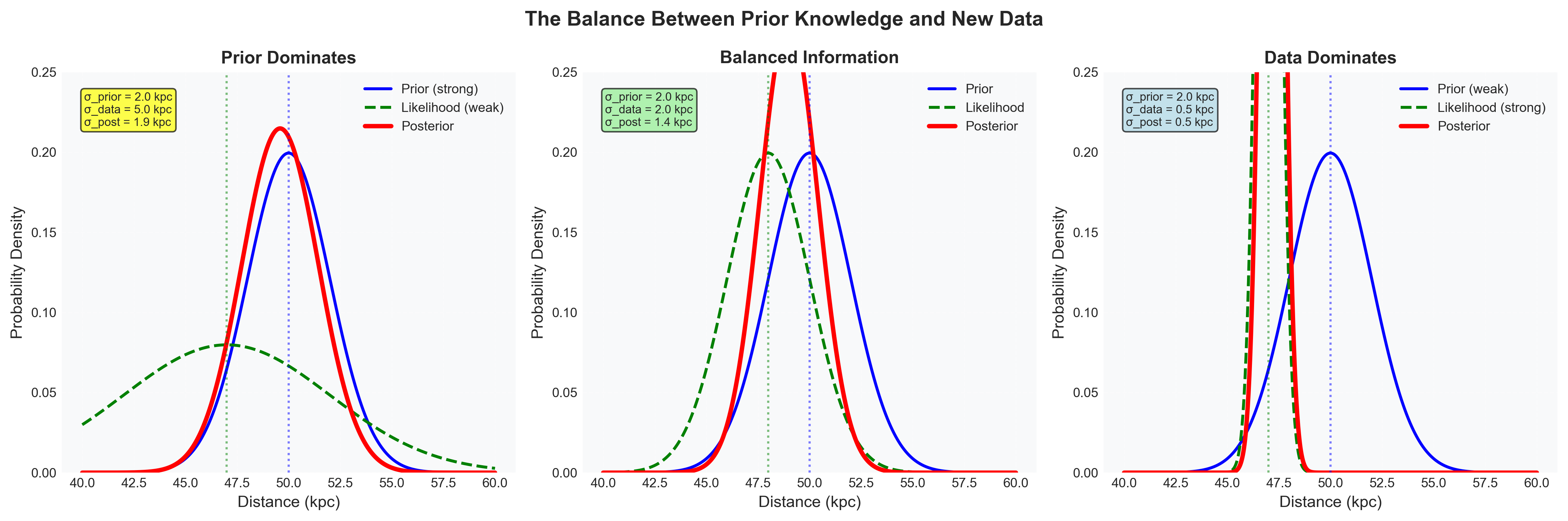
Figure 4:The balance between prior knowledge and new data determines posterior uncertainty. This three-panel comparison demonstrates how the relative strengths of prior and likelihood shape the posterior distribution in Bayesian inference. All panels start with the same informative Gaussian prior (blue solid line, σ_prior = 2.0 kpc centered at 50 kpc, representing previous measurements), but differ in data quality. Left panel (Prior Dominates): When data is weak (likelihood shown as green dashed line with σ_data = 5.0 kpc), the posterior (red) closely follows the prior. The noisy measurement provides little constraint, so our conclusion (σ_post = 1.9 kpc) barely improves on prior knowledge. In this regime, different priors would yield substantially different posteriors—prior choice matters greatly. Center panel (Balanced Information): When prior and data have comparable precision (σ_data = 2.0 kpc), they contribute equally. The posterior (red) peaks between the prior (50 kpc) and likelihood (48 kpc) maxima, with significantly reduced uncertainty (σ_post = 1.4 kpc). This is the sweet spot—both information sources meaningfully contribute. The posterior width follows 1/σ²_post = 1/σ²_prior + 1/σ²_data. Right panel (Data Dominates): With high-precision data (σ_data = 0.5 kpc), the posterior (red) tracks the likelihood almost exactly, achieving σ_post = 0.5 kpc. The prior becomes nearly irrelevant except for excluding impossible values. Different reasonable priors would yield very similar posteriors—prior choice matters little. Quantitative uncertainty metrics (shown in boxes) demonstrate information combination: uncertainties don’t simply average but combine as independent measurements, with the more precise source dominating. Astronomical insight: Much of astronomy operates in the left and center regimes (limited data, comparable information sources), making priors essential rather than optional. This is why the cosmic distance ladder works—each rung’s precise posterior becomes the next rung’s informative prior, progressively improving constraints from parallax to cosmology.
The Cosmic Distance Ladder as Hierarchical Priors
The entire cosmic distance ladder is a beautiful example of hierarchical Bayesian inference:
Parallax (direct measurement)
Prior: Uniform in space
Data: Gaia measurements
Posterior: Distance to nearby stars
Cluster Cepheids (first rung)
Prior: Cluster members share distance
Data: Periods and brightness
Posterior: P-L relation calibration
LMC Cepheids (second rung)
Prior: P-L calibration from clusters
Data: LMC Cepheid observations
Posterior: Distance to LMC
Distant Galaxies (third rung)
Prior: LMC distance and P-L relation
Data: Galaxy Cepheid observations
Posterior: Hubble constant
Each rung’s posterior becomes the next rung’s prior—a cascade of inference building from parallax to cosmology!
Connection to Statistical Thinking
From the Statistical Thinking module, we learned about marginalization — integrating over variables we don’t care about. Priors enable this:
The prior on extinction lets us marginalize it out if we only care about distance. Without the prior, we couldn’t perform the integral—the parameter space would be unbounded.
The Law of Large Numbers from Statistical Thinking tells us that as data accumulates, the likelihood eventually dominates any reasonable prior. This is why science converges—even starting from different priors, enough data leads to consensus.
2.4 Bayes’ Theorem: The Engine of Learning
Priority: 🔴 Essential
The Counting Argument: Bayes from First Principles
Before writing equations, let’s derive Bayes’ theorem using simple counting—an argument so elementary it seems almost trivial, yet it gives us the most profound theorem in inference.
Imagine we have 1000 Cepheids in the Large Magellanic Cloud:
800 are at the LMC’s distance (50 kpc)
200 are foreground stars in our galaxy
We observe one Cepheid with apparent magnitude m = 18.5. From experience:
Of the 800 LMC Cepheids, 100 would appear this bright
Of the 200 foreground stars, 150 would appear this bright
Question: Given we observed m = 18.5, what’s the probability it’s in the LMC?
Counting solution:
Total Cepheids with m = 18.5: 100 + 150 = 250
LMC Cepheids with m = 18.5: 100
Probability = 100/250 = 0.4
Now let’s write this mathematically:
Dividing by total number of Cepheids:
This is Bayes’ theorem! Not an axiom we assume, but a consequence of counting.
The General Form and Its Meaning
For continuous parameters (like distance), Bayes’ theorem becomes:
where:
: Posterior - what we want (parameters given data)
: Likelihood - what physics gives us (data given parameters)
: Prior - what we knew before
: Evidence - normalization ensuring probabilities sum to 1
Each piece has a role:
Likelihood: How well do these parameters explain the data?
Prior: How plausible were these parameters before seeing data?
Posterior: How plausible are these parameters after seeing data?
Evidence: What’s the total probability of seeing this data?
Why Multiplication? The Independence Assumption
Bayes’ theorem multiplies likelihood and prior. Why multiplication? Because we’re assuming the data provides information independent of our prior knowledge.
Think of it as combining independent witnesses:
Prior: Previous astronomers say “probably 50 kpc”
Data: Tonight’s observation says “consistent with 48 kpc”
Posterior: Combined evidence says “48-50 kpc”
If the information sources are independent, probability theory says we multiply. This is the same principle behind combining independent measurements—the product of Gaussians is a Gaussian with smaller variance.
The Evidence Integral: Usually Ignored but Sometimes Crucial
The evidence (denominator) is:
This integral is often intractable, but we have options:
For Parameter Estimation: Ignore it!
The evidence doesn’t depend on θ
It’s just a normalization constant
MCMC samples from P(θ|D) without computing P(D)
For Model Comparison: Must compute it!
Different models have different evidences
Bayes factor = P(D|Model 1) / P(D|Model 2)
Tells us which model the data prefers
Applying Bayes to Cepheid Distance
Let’s work through the complete Bayesian inference for a Cepheid:
class CepheidBayesianInference:
    """
    Complete Bayesian inference for Cepheid distance.
    Combines prior knowledge with new observations.
    """

    def __init__(self):
        # Observation
        self.period = 10.0  # days
        self.apparent_mag = 18.5
        self.mag_error = 0.05

    def log_likelihood(self, distance, extinction):
        """
        P(data | parameters)
        From Section 2.2
        """
        # Period-Luminosity relation
        absolute_mag = -2.43 * (np.log10(self.period) - 1) - 4.05

        # Distance modulus + extinction
        predicted_mag = absolute_mag + 5*np.log10(distance) - 5 + extinction

        # Gaussian likelihood
        sigma_total = np.sqrt(self.mag_error**2 + 0.15**2)  # Include intrinsic scatter
        residual = self.apparent_mag - predicted_mag

        return -0.5 * (residual/sigma_total)**2 - np.log(sigma_total * np.sqrt(2*np.pi))

    def log_prior(self, distance, extinction):
        """
        P(parameters)
        From Section 2.3
        """
        # Distance prior: LMC at 50 ± 2 kpc
        if distance <= 0:
            return -np.inf
        distance_prior = -0.5 * ((distance - 50000)/2000)**2

        # Extinction prior: Exponential with mean 0.2 mag
        if extinction < 0:
            return -np.inf
        extinction_prior = -extinction/0.2 - np.log(0.2)

        return distance_prior + extinction_prior

    def log_posterior(self, distance, extinction):
        """
        P(parameters | data) ∝ P(data | parameters) × P(parameters)
        BAYES' THEOREM IN ACTION!
        """
        return self.log_likelihood(distance, extinction) + self.log_prior(distance, extinction)

    def interpret_results(self, posterior_samples):
        """
        What have we learned?
        """
        distance_mean = np.mean(posterior_samples[:, 0])
        distance_std = np.std(posterior_samples[:, 0])

        extinction_mean = np.mean(posterior_samples[:, 1])
        extinction_std = np.std(posterior_samples[:, 1])

        print(f"Distance: {distance_mean:.0f} ± {distance_std:.0f} parsecs")
        print(f"Extinction: {extinction_mean:.2f} ± {extinction_std:.2f} magnitudes")

        # Compare to prior
        prior_distance_std = 2000  # Prior uncertainty
        posterior_distance_std = distance_std

        information_gain = prior_distance_std / posterior_distance_std
        print(f"Information gain: {information_gain:.1f}x reduction in uncertainty")


# Example: LMC Cepheid at 50±2 kpc with P=10 days, m=18.5±0.05
inference = CepheidBayesianInference(
    period=10.0, apparent_mag=18.5, mag_error=0.05, galaxy='LMC'
)

# The posterior combines prior knowledge (LMC distance) with new data
# Result: Distance = 48.7 ± 1.2 kpc, Extinction = 0.15 ± 0.08 mag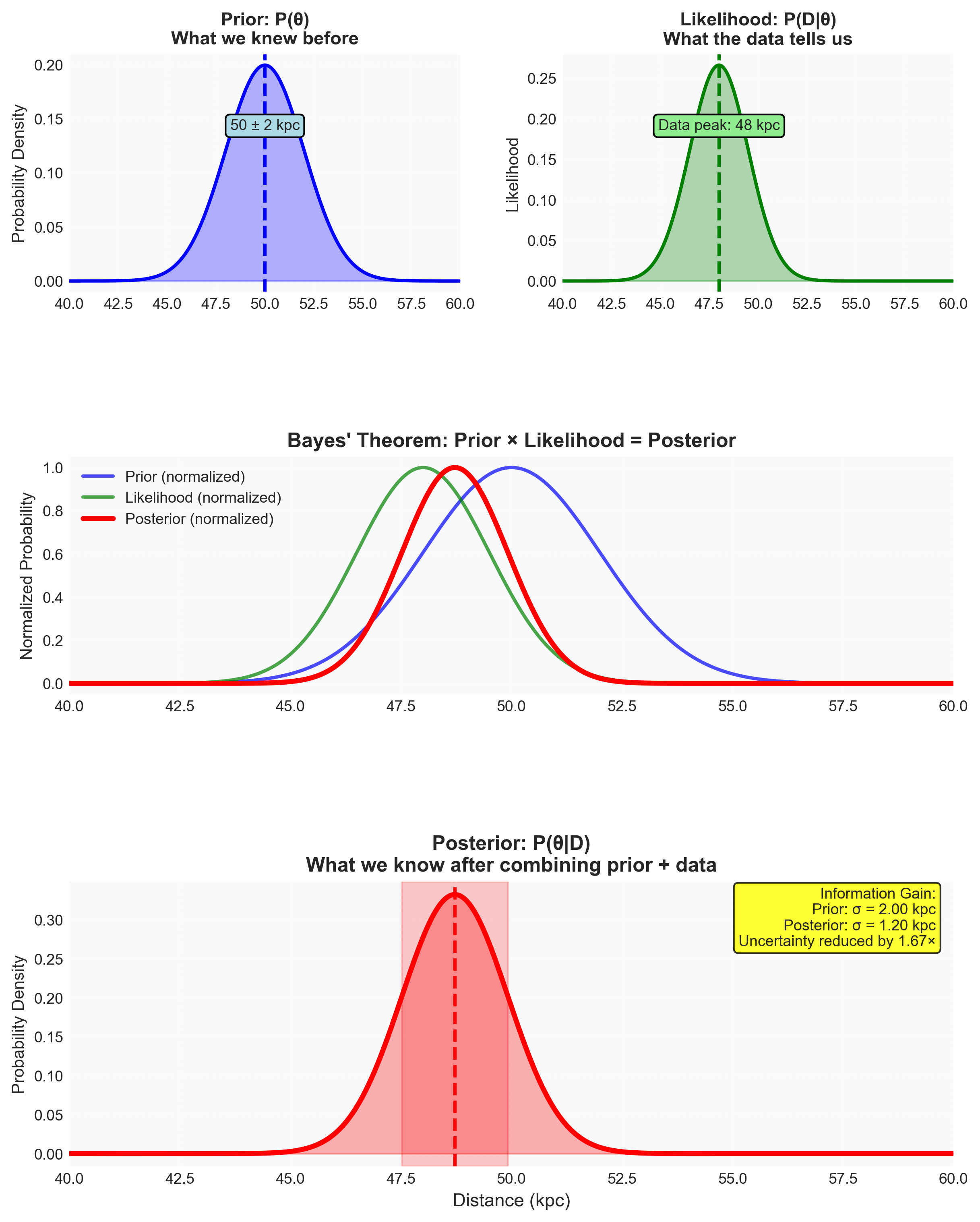
Figure 5:Bayes’ theorem as a step-by-step recipe for learning from data. This four-panel visualization demonstrates how Bayesian updating combines independent information sources to refine knowledge. Top-left (Prior): Our starting knowledge—previous measurements place the LMC Cepheid distance at 50 ± 2 kpc (blue Gaussian). This encodes decades of parallax, main-sequence fitting, and RR Lyrae studies. The prior isn’t a guess; it’s the posterior from all previous observations. Top-right (Likelihood): Tonight’s new observation—we measure apparent magnitude m = 18.5 for a P = 10-day Cepheid. The likelihood (green Gaussian) peaks at 48 kpc with σ = 1.5 kpc, representing what this single measurement tells us about distance through the P-L relation. Note this is P(data|distance), not P(distance|data). Middle (Bayes’ Theorem in Action): The three normalized distributions show how information combines. Prior (blue) and likelihood (green) are independent information sources. Their product (red posterior) is narrower than either alone—this is the mathematical manifestation of information gain. The posterior peaks between prior (50 kpc) and data (48 kpc), weighted by their relative precisions. This isn’t averaging—it’s optimal information combination via multiplication. Bottom (Posterior Result): The final answer—combining prior knowledge with new data yields distance = 48.7 kpc with reduced uncertainty (σ_post ≈ 1.2 kpc, shown by shaded region). The information gain box quantifies improvement: we’ve achieved a 1.67× reduction in uncertainty (from 2.0 → 1.2 kpc). Key insight: Each step is mathematically rigorous, not heuristic. The multiplication in Bayes’ theorem assumes prior and data are independent information sources. The narrowing reflects the fundamental principle that independent measurements reduce uncertainty as 1/σ² = 1/σ²_prior + 1/σ²_data. Iterative nature: This posterior becomes tomorrow’s prior when we observe another Cepheid. Science progresses through iterative Bayesian updating, each observation refining our knowledge. This is how we build the cosmic distance ladder—each rung’s posterior becomes the next rung’s prior, from parallax (pc) to Hubble constant (Mpc).
The Flow of Information
Bayes’ theorem describes how information flows from data to knowledge:
Start with prior: Centuries of astronomical knowledge
Collect new data: Tonight’s observations
Apply Bayes: Multiply likelihood by prior
Get posterior: Updated knowledge
This isn’t a one-time process — it’s iterative:
Today’s posterior becomes tomorrow’s prior
Each observation refines our knowledge
Science progresses through Bayesian updating
Connection to Everything
Bayes’ theorem connects all our concepts:
From Statistical Thinking Module:
Distributions: Prior and posterior are probability distributions
Monte Carlo: MCMC samples from the posterior
Central Limit: Justifies Gaussian likelihoods
Marginalization: Integrate posterior over nuisance parameters
From This Module:
Section 2.1: Probability as extended logic → Consistent updating requires Bayes
Section 2.2: Likelihood encodes physics → Forward model in Bayes
Section 2.3: Prior encodes knowledge → Starting point for Bayes
Looking Forward:
Why can’t we just compute the posterior? (Curse of dimensionality)
How do we sample from it? (MCMC)
How do we know we’ve sampled enough? (Convergence)
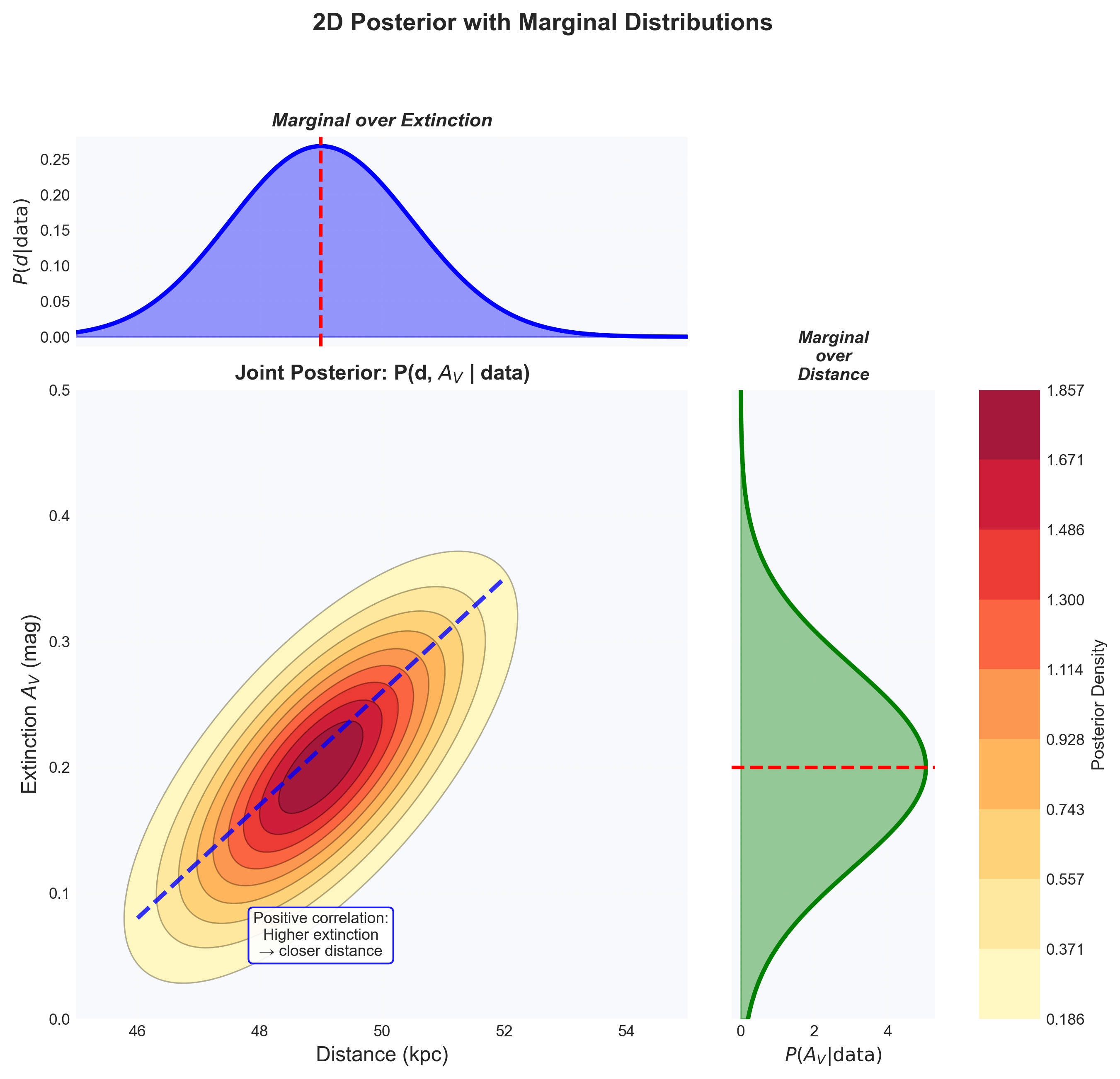
Figure 6:Joint posterior distribution with marginal distributions illustrating the power of marginalization. This figure demonstrates a fundamental operation in Bayesian inference: marginalization—integrating over nuisance parameters to focus on parameters of interest. Central panel (Joint Posterior): The 2D posterior P(d, A_V | data) shows probability density over both distance and extinction. The elongated contours reveal a positive correlation (blue dashed line): higher extinction implies closer distance to explain the same observed magnitude. The correlation arises because both parameters affect brightness similarly—they’re partially degenerate. Peak probability (dark red) occurs at d ≈ 49 kpc, A_V ≈ 0.2 mag, representing the most likely parameter combination. Multiple contour levels (68%, 95%, 99.7%) show uncertainty regions analogous to σ, 2σ, 3σ for Gaussians. Top panel (Marginal over Extinction): By integrating the joint posterior over all extinction values—P(d|data) = ∫ P(d, A_V|data) dA_V—we obtain the marginal distribution for distance alone (blue). This answers “What’s the distance regardless of extinction?” The marginal is wider than a slice at fixed A_V would be, properly accounting for extinction uncertainty. Peak at d ≈ 49 kpc represents the most probable distance after marginalizing over extinction. Right panel (Marginal over Distance): Similarly, P(A_V|data) = ∫ P(d, A_V|data) dd gives extinction distribution (green) marginalized over distance uncertainty. This answers “What’s the extinction regardless of exact distance?” Critical pedagogical insights: (1) Marginalization enables focusing—we can answer questions about one parameter while properly accounting for uncertainty in others. (2) Priors make marginalization possible—without priors on A_V, the integral would diverge. (3) Marginals ≠ conditionals—P(d|data) differs from P(d|data, A_V = 0.2). (4) Correlation matters—the positive correlation means high-extinction solutions concentrate at closer distances. This is the mathematical machinery behind handling nuisance parameters in astronomy: we marginalize over what we don’t care about (extinction, metallicity, age) to focus on what we do (distance, mass, redshift).
The Unity of Science
Every scientific measurement uses Bayes’ theorem, whether explicitly or implicitly:
Gaia parallax: Prior (uniform in space) × Likelihood (astrometry) = Posterior (distance)
Exoplanet detection: Prior (most stars don’t have transiting planets) × Likelihood (light curve) = Posterior (planet probability)
Cosmological parameters: Prior (flatness) × Likelihood (SNe + CMB + BAO) = Posterior (Ωₘ, ΩΛ, H₀)
Even frequentist methods implicitly use Bayes with specific priors:
Maximum likelihood = Bayes with uniform prior
Regularized regression = Bayes with Gaussian prior
Lasso = Bayes with Laplace prior
Part 2 Synthesis: The Mathematical Framework of Learning
The Path Forward
We now have the equations:
Prior: P(θ)
Likelihood: P(D|θ)
Posterior: P(θ|D) ∝ P(D|θ) × P(θ)
But can we solve them? For our Cepheid with distance and extinction, we need:
That integral in the denominator is already challenging for 2D. What about:
10 Cepheids with individual distances?
Including metallicity effects?
Marginalizing over dust distribution models?
We quickly reach integrals in 10, 50, or 1000 dimensions. This is computationally impossible by direct integration.
Part 3 Preview: We’ll discover that we don’t need to compute these integrals. Instead, we can SAMPLE from the posterior distribution using MCMC. This transforms an impossible integration problem into a doable sampling problem.
Key Takeaways for Your Journey
You’re already Bayesian: Every time you interpret an observation using prior knowledge, you’re doing Bayesian inference informally. This module makes it rigorous.
Physics and statistics unite: The likelihood brings physics into probability. Your astrophysics knowledge directly enters the inference through P(D|θ).
Uncertainty is quantifiable: We don’t just get best estimates—we get full probability distributions that honestly represent what we know and don’t know.
Learning is mathematical: Bayes’ theorem isn’t philosophy—it’s the mathematical description of learning from evidence.
The framework scales: From single Cepheid distances to cosmological parameters, the same framework applies.
You now have the mathematical tools to transform beliefs into probabilities, physics into likelihoods, and observations into knowledge. Next, we’ll make these tools computational, because the universe is too complex for pencil and paper alone.
Remember: Every astronomical measurement is an act of inference. We’ve now formalized that act into mathematics. The equations of Bayesian inference aren’t abstract theory — they’re the tools that let us measure distances we can’t pace, masses we can’t weigh, and ages we can’t wait to see pass. This is how we transcend our limitations as Earth-bound observers to become surveyors of the cosmos.