Chapter 2: Python as Your Scientific Calculator
Modeling the Universe | Python Fundamentals
Learning Objectives
By the end of this chapter, you will be able to:
(1) Use Python as an interactive scientific calculator with correct operator precedence (PEMDAS) and all seven arithmetic operators (
+,-,*,/,//,%,**).(2) Explain how computers represent numbers in memory using IEEE 754 standard for floats (64 bits: sign, exponent, mantissa) and arbitrary precision for integers.
(3) Demonstrate why
0.1 + 0.2 ≠ 0.3due to binary representation limits and handle comparisons withmath.isclose().(4) Recognize and prevent three numerical hazards: catastrophic cancellation, overflow (~10³⁰⁸ limit), and silent underflow to zero.
(5) Choose appropriate numeric types (int, float32, float64, complex) based on precision needs and memory constraints.
(6) Format scientific output using f-strings with format specifiers (
.2f,.2e,:10.2f,:,) for publication-quality results.(7) Convert between data types safely using
int(),float(),complex()while understanding truncation vs rounding.(8) Apply defensive programming techniques including validation functions, safe division, and domain-specific checks.
(9) Use essential
mathmodule functions for scientific computing:sqrt(),log(),sin(),cos(),isfinite(),isnan().(10) Work with complex numbers using Python’s
jnotation for wave physics and Fourier analysis.
Prerequisites Check
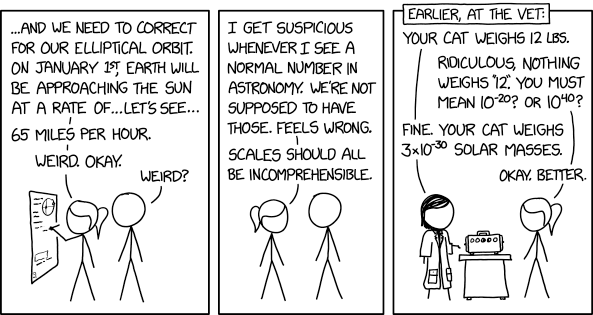
Sometimes the universe writes better stories than we could imagine. (xkcd)
Chapter Overview
Now that you’ve mastered setting up your computational environment and understand how Python finds and loads code, it’s time to transform IPython into your personal calculator. But this chapter goes far beyond simple arithmetic - you’re about to discover the hidden complexity of numerical computation that can make the difference between discovering an exoplanet and missing it entirely due to rounding errors.
You’ll learn why spacecraft have crashed, why some astronomical calculations fail catastrophically, and how to write code that handles the extreme scales of the universe — from the quantum foam at meters to the observable universe at meters. The floating-point precision issues we explore here aren’t academic exercises; they’re the source of real bugs that have corrupted simulations, invalidated published results, and caused spacecraft navigation errors costing hundreds of millions of dollars.
By mastering these fundamentals now, you’ll develop the numerical intuition that separates computational scientists from programmers who just happen to work with scientific data. Every orbital integrator you build, every spectrum you analyze, and every statistical test you run will rely on the concepts in this chapter. Let’s begin your journey from calculator user to numerical computing expert.
2.1 Python as Your Scientific Calculator
Fire up ipython (remember from Chapter 1 — not the basic python interpreter, we want the enhanced features) and let’s start with the basics. Python handles arithmetic operations naturally, but there are subtleties that matter for scientific work:
# Basic arithmetic - but watch the precision!
print(f"2 + 2 = {2 + 2}")
print(f"10 / 3 = {10 / 3}")  # Division always gives a float
print(f"2 ** 10 = {2 ** 10}")  # Exponentiation - the power operator
Notice that 10 / 3 gives us 3.3333333333333335 — not exactly 1/3! This tiny imprecision at the end might seem trivial, but it’s your first glimpse into a fundamental challenge of computational science.
Operator Precedence: A Source of Real Bugs
Python follows PEMDAS (Parentheses, Exponents, Multiplication/Division, Addition/Subtraction), but relying on memorized rules causes expensive errors. Let’s see this with a real astronomical calculation:
# Calculate orbital velocity: v = sqrt(GM/r)
# Using CGS units (standard in astrophysics)
G = 6.67e-8   # Gravitational constant (cm³ g⁻¹ s⁻²)
M = 1.989e33  # Solar mass (grams)
r = 1.496e13  # 1 AU (cm)

# WRONG - operator precedence error!
v_wrong = G * M / r ** 0.5
print(f"Wrong velocity: {v_wrong:.2e} cm/s")

# CORRECT - parentheses clarify intent
v_right = (G * M / r) ** 0.5
print(f"Correct velocity: {v_right:.2e} cm/s")
print(f"That's {v_right/1e5:.1f} km/s - Earth's orbital speed!")

# The error factor
error_factor = v_wrong / v_right
print(f"Wrong answer is {error_factor:.0f}× too large!")The wrong version calculated instead of — a factor of error, which for Earth’s orbit is about 1013 times too large!
Solution
Let’s work through -2**2 + 3*4//2 step by step:
Exponentiation first:
2**2 = 4Then negation:
-4(the negative applies after exponentiation!)Multiplication:
3*4 = 12Floor division:
12//2 = 6Finally addition:
-4 + 6 = 2
The result is 2. The tricky part is that -2**2 equals -4, not 4! Python interprets this as -(2**2), not (-2)**2. This subtle precedence rule has caused real bugs in astronomical calculations.
Complete Arithmetic Operators
Python provides operators beyond basic arithmetic that prove essential for astronomical calculations:
# Integer division - useful for time calculations
days = 17
weeks = days // 7  # Floor division
remaining_days = days % 7  # Modulo (remainder)
print(f"{days} days = {weeks} weeks and {remaining_days} days")

# Warning: Floor division rounds toward negative infinity!
print(f"17 // 3 = {17 // 3}")    # Result: 5
print(f"-17 // 3 = {-17 // 3}")  # Result: -6, not -5!

# This catches many astronomers by surprise
print("\nBe careful with negative values:")
print(f"int(-17/3) = {int(-17/3)} (truncates toward zero)")
print(f"-17 // 3 = {-17 // 3} (floors toward -infinity)")2.2 How Python Stores Numbers: Critical for Scientific Computing
Here’s where your journey gets interesting! You’re about to peek behind the curtain and see how computers really think about numbers. This knowledge is your superpower — it’s what lets you calculate the trajectory to send New Horizons to Pluto, 3 billion miles away, and arrive within 72 seconds of the predicted time.
Integers: Arbitrary Precision Power
Unlike many languages, Python integers have unlimited precision — a huge advantage for astronomy where we routinely deal with enormous numbers:
# Number of atoms in the observable universe (approximate)
atoms_in_universe = 10 ** 80
print(f"Atoms in universe: {atoms_in_universe}")

# Python handles it perfectly!
atoms_squared = atoms_in_universe ** 2
print(f"Can even square it: {atoms_squared}")

# Memory usage scales with size
import sys
print(f"\nMemory usage comparison:")
print(f"Small integer (42) uses: {sys.getsizeof(42)} bytes")
print(f"Universe atoms uses: {sys.getsizeof(atoms_in_universe)} bytes")
print(f"Atoms squared uses: {sys.getsizeof(atoms_squared)} bytes")
This arbitrary precision is wonderful but comes with a cost — Python integers use more memory than fixed-size integers in compiled languages. This is why specialized numerical libraries become essential for large datasets.
Floating-Point Numbers: The Heart of Numerical Computing
This is it — the concept that separates casual programmers from computational scientists! Don’t worry if this seems complex at first; every professional scientist had to learn these same lessons.
Floating-point numbers use IEEE 754 representation: 64 bits split into sign (1 bit), exponent (11 bits), and mantissa (52 bits). This creates fundamental limitations that every computational scientist must understand.
Understanding Bits and Precision
Before diving into floating-point challenges, let’s understand the fundamental unit of computer memory: the bit. A bit (binary digit) can store exactly one of two values: 0 or 1. Think of it as a light switch—either on or off. Everything your computer does ultimately reduces to manipulating billions of these tiny switches.
Groups of bits form larger units:
8 bits = 1 byte (can represent 256 different values: 2⁸)
32 bits = 4 bytes (can represent ~4.3 billion values: 2³²)
64 bits = 8 bytes (can represent ~18 quintillion values: 2⁶⁴)
Single vs Double Precision: The 32-bit vs 64-bit Choice
Floating-point numbers come in two main flavors:
import numpy as np
import sys

# Python's default float is 64-bit (double precision)
regular_float = 3.14159265358979323846
print(f"Python float: {sys.getsizeof(regular_float)} bytes")
print(f"Precision: {regular_float}")

# NumPy lets us choose 32-bit (single precision)
single_precision = np.float32(3.14159265358979323846)
double_precision = np.float64(3.14159265358979323846)

print(f"\n32-bit representation: {single_precision}")
print(f"64-bit representation: {double_precision}")
print(f"Lost digits in 32-bit: {double_precision - single_precision:.10e}")

# Where do those bits go?
print("\nIEEE 754 Standard bit allocation:")
print("32-bit: 1 sign + 8 exponent + 23 mantissa bits")
print("64-bit: 1 sign + 11 exponent + 52 mantissa bits")
The trade-offs are crucial for scientific computing:
| Aspect | 32-bit (float32) | 64-bit (float64) |
|---|---|---|
| Precision | ~7 decimal digits | ~15 decimal digits |
| Range | ±10⁻³⁸ to 10³⁸ | ±10⁻³⁰⁸ to 10³⁰⁸ |
| Memory | 4 bytes | 8 bytes |
| Speed | Faster on GPU | Standard on CPU |
| Use case | Graphics, ML training | Scientific computing |
# Precision matters for astronomical calculations!
import math

# Distance to Proxima Centauri in meters
distance_m = 4.0e16

# Small measurement error
error_32bit = distance_m * np.float32(1.0000001) - distance_m
error_64bit = distance_m * np.float64(1.0000001) - distance_m

print(f"Measurement error with 32-bit: {error_32bit:.0f} meters")
print(f"Measurement error with 64-bit: {error_64bit:.0f} meters")
print(f"Difference: {abs(error_32bit - error_64bit):.0f} meters")
print(f"That's {abs(error_32bit - error_64bit)/1000:.0f} km of error!")
Python defaults to 64-bit because scientific computing needs that precision. But libraries like JAX default to 32-bit for machine learning where speed matters more than precision. For numerical computing with JAX, you can configure it to use 64-bit precision by setting jax.config.update('jax_enable_x64', True) at the start of your program. Always know which precision you’re using!
⚠️ 🌟 The More You Know: Why Quantum Computers Could Change Everything
While your classical computer uses bits that must be either 0 or 1, quantum computers use qubits that can exist in superposition—simultaneously 0 and 1 until measured. This isn’t just a faster bit; it’s fundamentally different.
Classical bit: Like a coin that’s either heads OR tails Qubit: Like a spinning coin that’s both heads AND tails until it lands
This superposition enables quantum parallelism:
Classical: To try 1,000 possibilities, do 1,000 calculations sequentially
Quantum: Try all 1,000 possibilities simultaneously in superposition
Why it matters for astronomy:
Simulation: A classical computer needs 2ⁿ bits to perfectly simulate n qubits. Just 300 qubits would require more classical bits than there are atoms in the universe!
Optimization: Finding optimal telescope scheduling among millions of targets, or searching for patterns in cosmological data, could be exponentially faster.
Many-body problems: Simulating quantum systems (like stellar interiors or the early universe) naturally—quantum systems simulating quantum physics.
The catch? Qubits are incredibly fragile. Current quantum computers need to be cooled to near absolute zero and isolated from all vibrations. A single cosmic ray can destroy a calculation. Google’s 2019 “quantum supremacy” demonstration used 53 qubits for just 200 seconds of computation.
Current reality (2024): Quantum computers excel at specific tasks (cryptography, optimization, quantum simulation) but can’t run Python or browse the web. They’re specialized tools, not general-purpose computers. IBM, Google, and others offer cloud access to real quantum computers you can experiment with today!
The dream? Hybrid systems where quantum processors handle what they do best (optimization, simulation) while classical computers handle everything else. Your orbital mechanics simulation might one day use quantum algorithms to find optimal trajectories, then classical computing to visualize the results.
For now, we’re stuck with bits—but understanding their limitations helps us write better code within those constraints!
Back to Classical Reality: Why 0.1 + 0.2 ≠ 0.3
Now that you understand bits and precision, let’s see why even 64-bit floats can’t exactly represent simple decimals.
# The famous example that confuses beginners
result = 0.1 + 0.2
print(f"0.1 + 0.2 = {result}")
print(f"0.1 + 0.2 == 0.3? {result == 0.3}")
print(f"Actual stored value: {result:.17f}")

# Let's see what's really stored
from decimal import Decimal
print(f"\nWhat Python actually stores:")
print(f"0.1 is really: {Decimal(0.1)}")
print(f"0.2 is really: {Decimal(0.2)}")
print(f"0.3 is really: {Decimal(0.3)}")
Why does this happen? Just as 1/3 can’t be exactly represented in decimal (0.33333...), 1/10 can’t be exactly represented in binary. This has crashed spacecraft and corrupted years of simulations!
Solution
This returns False! Here’s why:
print(f"0.1 * 3 = {0.1 * 3:.17f}")
print(f"0.3 =     {0.3:.17f}")
You’ll see that 0.1 * 3 gives approximately 0.30000000000000004, while 0.3 is approximately 0.29999999999999999. They’re different by about - tiny but not zero!
This isn’t a quirk — it’s fundamental to how every computer on Earth handles decimals. This is why we always use math.isclose() for floating-point comparisons.
Machine Epsilon: The Smallest Distinguishable Difference
Ready for something mind-blowing? Your computer literally cannot tell the difference between some numbers that are mathematically different! This isn’t a flaw — it’s a fundamental property of finite systems.
import sys

# Machine epsilon - the fundamental precision limit
epsilon = sys.float_info.epsilon
print(f"Machine epsilon: {epsilon}")
print(f"That's about {epsilon:.2e}")

# Numbers closer than epsilon to 1.0 cannot be distinguished
test1 = 1.0 + epsilon/2
test2 = 1.0 + epsilon

print(f"\nCan Python tell these apart from 1.0?")
print(f"1.0 + ε/2 = {test1}, equals 1.0? {test1 == 1.0}")
print(f"1.0 + ε   = {test2}, equals 1.0? {test2 == 1.0}")

# This affects astronomical calculations
au_cm = 1.496e13  # 1 AU in centimeters
tiny_change = au_cm * epsilon
print(f"\nAt 1 AU distance ({au_cm:.2e} cm):")
print(f"We cannot detect changes smaller than {tiny_change:.2e} cm")
print(f"That's about {tiny_change/100:.2f} meters!")
When the Kepler Space Telescope searched for exoplanets by detecting brightness dips of 0.01%, understanding machine epsilon was essential to distinguish real planetary transits from numerical noise.
⚠️ 💥 Why This Matters: The Patriot Missile Timing Disaster
On February 25, 1991, an American Patriot missile battery in Dhahran, Saudi Arabia, failed to intercept an incoming Iraqi Scud missile. The Scud struck an Army barracks, killing 28 soldiers and injuring 98 others. The cause? A tiny numerical error that accumulated over time.
The Patriot’s targeting system tracked time using a 24-bit fixed point register, counting in tenths of seconds. However, 1/10 has no exact binary representation—in 24-bit precision, the stored value was actually 0.099999904632568359375, creating an error of approximately 0.000000095 seconds per tenth of a second.
After running continuously for 100 hours (360,000 tenth-second increments), this microscopic error had grown to:
Timing error: 0.34 seconds
Range gate error: ~687 meters (Scud velocity ≈ 2,000 m/s)
The Patriot radar system looked in the wrong section of sky and never detected the incoming missile.
The bitter irony? Israeli forces had already noticed targeting problems after 8 hours of continuous operation. A software patch had been written, and was literally in transit to Dhahran when the attack occurred. The original design specification called for maximum 14-hour operation periods—nobody anticipated 100 hours of continuous use.
The lesson for scientific computing: Even “negligible” rounding errors become significant when accumulated over many iterations. Whether you’re integrating orbits over millions of timesteps or tracking particles in a simulation, always consider:
How errors propagate through iterations
Whether your precision is adequate for the timescales involved
The difference between relative and absolute error tolerances
[Source: GAO Report IMTEC-92-26, Skeel, R. (1992). “Roundoff Error and the Patriot Missile.” SIAM News]
Safe Floating-Point Comparisons
Never use == with floating-point numbers! Here’s how to compare them safely:
Stage 1: Understanding the Problem
# The problem with direct comparison
velocity = 299792458.0  # Speed of light in m/s
calculated = 299792457.999999999  # From some calculation

print(f"Velocity: {velocity}")
print(f"Calculated: {calculated}")
print(f"Difference: {velocity - calculated:.2e}")
print(f"Are they equal? {velocity == calculated}")
print("Even tiny differences fail equality test!")
Stage 2: Basic Solution
def safe_compare_simple(a, b, tolerance=1e-9):
    """Compare floats with absolute tolerance."""
    difference = abs(a - b)
    return difference <= tolerance

# Test our function
v1 = 299792458.0
v2 = 299792457.999999999

result = safe_compare_simple(v1, v2, tolerance=1e-6)
print(f"Within tolerance? {result}")
Stage 3: Professional Solution
import math

def safe_compare(a, b, rel_tol=1e-9, abs_tol=1e-15):
    """Compare floats safely with relative and absolute tolerance."""
    # Handle special cases
    if math.isnan(a) or math.isnan(b):
        return False
    if math.isinf(a) or math.isinf(b):
        return a == b

    # Use relative and absolute tolerance
    return abs(a - b) <= max(rel_tol * max(abs(a), abs(b)), abs_tol)

# Better - use Python's built-in (available since Python 3.5)
result = math.isclose(v1, v2, rel_tol=1e-9)
print(f"Using math.isclose: {result}")2.3 Numerical Hazards in Scientific Computing
You’ve mastered how Python stores numbers — now let’s see these concepts in action with real scientific calculations! This is where things get exciting: you’re about to learn the techniques that enabled Cassini to thread the gap between Saturn’s rings, that allow LIGO to detect gravitational waves smaller than a proton’s width, and that help the Event Horizon Telescope image black holes.
Catastrophic Cancellation: When Subtraction Destroys Precision
Here’s a numerical phenomenon that sounds scary but becomes manageable once you understand it! Catastrophic cancellation happens when you subtract nearly equal numbers, eliminating most significant digits and leaving only rounding errors.
Stage 1: The Problem
import math

# Computing 1 - cos(x) for small x (common in orbital calculations)
x = 1e-8  # Small angle in radians

# Direct computation - catastrophic cancellation!
cos_x = math.cos(x)
result_bad = 1 - cos_x
print(f"Direct: 1 - cos({x}) = {result_bad}")
print(f"This result is completely wrong!")
Stage 2: Understanding Why
# Let's see what's happening
print(f"cos({x}) = {cos_x:.20f}")
print(f"1.0 =      1.00000000000000000000")
print(f"Difference loses all significant digits!")

# The true value (from Taylor series)
true_value = x**2 / 2  # For small x, 1-cos(x) ≈ x²/2
print(f"\nTrue value: {true_value:.6e}")
print(f"Our result: {result_bad:.6e}")
print(f"Relative error: {abs(result_bad - true_value)/true_value:.1%}")
Stage 3: The Solution
# Better: use mathematical identity
# 1 - cos(x) = 2sin²(x/2)
result_good = 2 * math.sin(x/2) ** 2
print(f"Using identity: {result_good:.6e}")
print(f"True value:     {true_value:.6e}")
print(f"Much better! Error: {abs(result_good - true_value)/true_value:.2e}")

# This preserves precision for small angles
🌟 The More You Know: Mars Climate Orbiter’s $327 Million Mistake
The Mars Climate Orbiter was destroyed on September 23, 1999, when it entered Mars’ atmosphere at 57 kilometers altitude instead of the planned 140-226 kilometers. While the famous cause was a metric/imperial unit mix-up (Lockheed Martin used pound-force seconds while NASA used newton-seconds), the navigation software also struggled with numerical precision issues.
The spacecraft’s trajectory correction maneuvers involved calculating tiny velocity changes (often less than 1 m/s) while traveling at over 20,000 m/s. This requires computing the difference between nearly equal large numbers — exactly the catastrophic cancellation problem we just solved.
When you’re 400 million kilometers from Earth and need millimeter-per-second precision in velocity, every numerical trick matters. The MCO failure led NASA to implement much stricter numerical validation in all navigation software (NASA, 2000).
Overflow and Underflow in Astronomical Scales
Get ready to work with numbers that break normal intuition! Astronomy deals with scales that push Python to its limits — from subatomic particles in neutron stars to galaxy clusters spanning millions of light-years.
Stage 1: The Overflow Problem
# Calculating total luminosity
L_sun = 3.828e33  # Solar luminosity (erg/s)
n_stars_galaxy = 1e11  # Stars in a galaxy
n_galaxies = 2e12  # Galaxies in observable universe

# This might overflow!
try:
    # Try direct multiplication
    L_universe = L_sun * n_stars_galaxy * n_galaxies
    print(f"Universe luminosity: {L_universe:.2e} erg/s")
except OverflowError:
    print("Direct calculation overflowed!")
    print("Number too large for float representation")
Stage 2: The Solution - Working in Log Space
import math

# When direct calculation fails, work in log space
log_L_sun = math.log10(L_sun)
log_n_stars = math.log10(n_stars_galaxy)
log_n_galaxies = math.log10(n_galaxies)

# Add logarithms instead of multiplying
log_L_universe = log_L_sun + log_n_stars + log_n_galaxies

print(f"Universe luminosity: 10^{log_L_universe:.1f} erg/s")
print(f"That's 10^{log_L_universe:.1f} ergs every second!")

# For comparison, the Sun's lifetime energy output
log_sun_lifetime = math.log10(L_sun) + math.log10(3.15e7 * 1e10)  # 10 billion years
print(f"Sun's total lifetime output: 10^{log_sun_lifetime:.1f} ergs")Defensive Programming with Numerical Checks
You’ve seen the challenges — now here’s your toolkit for conquering them! Defensive programming might sound cautious, but it’s actually incredibly empowering. These validation techniques protect every major astronomical data pipeline.
Stage 1: Basic Validation (10 lines)
def validate_positive(value, name="value"):
    """Ensure value is positive."""
    if value <= 0:
        raise ValueError(f"{name} must be positive: {value}")
    return value

# Example use
mass = validate_positive(1.989e33, "stellar mass")
print(f"Valid mass: {mass:.2e} g")
Stage 2: Safe Division
def safe_divide(a, b, epsilon=1e-15):
    """Division with protection against near-zero denominators."""
    if abs(b) < epsilon:
        raise ValueError(f"Division by near-zero: {b:.2e}")
    return a / b

# Test with safe division
force = safe_divide(G * M, r * r)
print(f"Gravitational acceleration: {force:.2e} cm/s²")

# Would catch divide-by-zero before it happens
Stage 3: Complete Validation (15 lines)
import math

def validate_magnitude(value, name="value", max_exp=100):
    """Ensure value is reasonable for astronomical calculations."""
    if value == 0:
        return value

    if not math.isfinite(value):
        raise ValueError(f"{name} is not finite: {value}")

    log_val = abs(math.log10(abs(value)))
    if log_val > max_exp:
        raise ValueError(f"{name} has unreasonable magnitude: {value:.2e}")

    return value

# Test validation
test_value = validate_magnitude(L_sun, "luminosity", max_exp=50)
print(f"Validated luminosity: {test_value:.2e} erg/s")
Stage 4: Domain-Specific Validation
def validate_schwarzschild_input(mass_grams):
    """
    Validate mass for black hole calculations.
    Ensures physically reasonable values for computational stability.

    Args:
        mass_grams: Mass in grams

    Returns:
        float: Validated mass
    """
    MIN_MASS = 2e31  # ~0.01 solar masses (brown dwarf lower limit)
    MAX_MASS = 2e44  # ~10¹¹ solar masses (largest known black holes)

    if not MIN_MASS <= mass_grams <= MAX_MASS:
        raise ValueError(
            f"Mass {mass_grams:.2e} g outside physical range "
            f"[{MIN_MASS:.2e}, {MAX_MASS:.2e}]"
        )

    return mass_grams

# Test with realistic astrophysical masses
stellar_bh = validate_schwarzschild_input(10 * 1.989e33)  # 10 $M_{\odot}$
print(f"Stellar black hole mass valid: {stellar_bh:.2e} g")

try:
    # This would fail - too small for any collapsed object
    validate_schwarzschild_input(1e20)
except ValueError as e:
    print(f"Validation caught error: {e}")
2.4 Complex Numbers for Wave Physics
Welcome to one of the most elegant corners of mathematics! Complex numbers might sound intimidating, but they’re actually your gateway to understanding everything from stellar oscillations to gravitational waves. Python handles complex numbers as naturally as integers.
# Complex numbers in Python use 'j' for the imaginary unit
z = 3 + 4j
print(f"Complex number: {z}")
print(f"Real part: {z.real}")
print(f"Imaginary part: {z.imag}")
print(f"Magnitude: {abs(z)}")

# Euler's formula - the most beautiful equation in mathematics
import cmath
euler = cmath.exp(1j * math.pi)
print(f"\ne^(iπ) = {euler.real:.0f}")
print(f"Tiny imaginary part {euler.imag:.2e} is just rounding error")

# Phase calculation (useful for wave interference)
phase = cmath.phase(z)
print(f"\nPhase of {z}: {phase:.3f} radians")
print(f"That's {math.degrees(phase):.1f} degrees")
Complex numbers aren’t just mathematical abstractions — they’re essential for:
Fourier transforms (spectral analysis)
Quantum mechanics (wave functions)
Signal processing (interferometry)
Every spectrum you’ve ever seen from a telescope was processed using complex numbers!
🎯 Why This Matters: Fourier Transforms Reveal Hidden Periods
Complex numbers aren’t just mathematical elegance—they’re essential for discovering exoplanets! The Fourier transform, which relies entirely on complex exponentials, transforms time-series brightness measurements into frequency space, revealing hidden periodicities.
Real Research Application:
The Kepler Space Telescope monitored 150,000 stars continuously for 4 years, collecting brightness measurements every 30 minutes. That’s ~70,000 data points per star—over 10 billion measurements total! Finding periodic dimming (transiting planets) in this ocean of data requires Fourier analysis:
# Simplified exoplanet detection
import numpy as np

# Time series: brightness over time
time = np.linspace(0, 100, 10000)  # 100 days
# Hidden planet: 3.5 day period, 0.01% dimming
signal = 1.0 - 0.0001 * np.cos(2*np.pi*time/3.5)
# Add noise
noise = np.random.normal(0, 0.0005, len(time))
brightness = signal + noise

# Fourier transform uses complex exponentials
frequencies = np.fft.fftfreq(len(time), time[1]-time[0])
fft = np.fft.fft(brightness - np.mean(brightness))
power = np.abs(fft)**2  # Complex magnitude squared

# Peak in power spectrum reveals planet period!
peak_idx = np.argmax(power[1:len(power)//2]) + 1
planet_period = 1/frequencies[peak_idx]
print(f"Detected period: {planet_period:.2f} days")
Without complex numbers and Euler’s formula (e^(iωt) = cos(ωt) + i⋅sin(ωt)), we couldn’t efficiently search for the 2,788 confirmed exoplanets discovered by Kepler. Every periodogram you’ll ever compute—whether finding pulsation modes in stars, orbital periods in binaries, or rotation periods of stars—depends on complex arithmetic.
The bottom line: Master complex numbers now, because every time-series analysis technique you’ll learn builds on them!
2.5 Variables and Dynamic Typing
Now that you understand how Python represents numbers, let’s see how it manages them! Variables in Python are names that refer to objects, not containers that hold values. This distinction matters:
# Variables are references, not containers
stellar_mass = 1.989e33  # Solar mass in grams
solar_mass = stellar_mass  # Both names refer to the SAME number

print(f"stellar_mass: {stellar_mass:.2e} g")
print(f"solar_mass: {solar_mass:.2e} g")
print(f"Same object? {stellar_mass is solar_mass}")

# But numbers are immutable, so this is safe
stellar_mass = stellar_mass * 2  # Creates NEW number
print(f"\nAfter doubling stellar_mass:")
print(f"stellar_mass: {stellar_mass:.2e} g")
print(f"solar_mass (unchanged): {solar_mass:.2e} g")
Python is dynamically typed — variables can refer to any type of object:
# Dynamic typing in action
observation = 42  # Integer
print(f"Type: {type(observation).__name__}, Value: {observation}")

observation = 42.0  # Now a float
print(f"Type: {type(observation).__name__}, Value: {observation}")

observation = "42 measurements"  # Now a string
print(f"Type: {type(observation).__name__}, Value: {observation}")

# This flexibility is powerful but requires discipline
# In scientific code, changing types unexpectedly is usually a bug!
2.6 Strings and Scientific Output Formatting
Time to make your results shine! Clear output formatting isn’t just about aesthetics — it’s about scientific communication. The formatting skills you learn here will help you create publication-quality output.
# Basic f-string formatting
star_name = "Betelgeuse"
distance_pc = 400
luminosity = 1.2e5  # Solar luminosities

print(f"{star_name} is {distance_pc} light-years away")
print(f"Luminosity: {luminosity:.2e} Lsun")
Format Specifications for Scientific Data
F-strings support sophisticated formatting perfect for scientific output:
# Comprehensive formatting examples
value = 1234.56789

print(f"Fixed-point (2 decimals): {value:.2f}")
print(f"Scientific notation: {value:.2e}")
print(f"Width 10, 2 decimals: {value:10.2f}")
print(f"Thousands separator: {value:,.0f}")

# Create a formatted table of stellar data
stars = [
    ("Sirius", -1.46, 8.6),
    ("Canopus", -0.74, 310),
    ("Arcturus", -0.05, 37),
]

print(f"\n{'Star':<10} {'Magnitude':>10} {'Distance (ly)':>15}")
print("-" * 37)
for name, mag, dist in stars:
print(f"{name:<10} {mag:>10.2f} {dist:>15.1f}")Solution
This prints: z = 1.23e-03
The .2e format specifier means:
Use scientific notation (e)
Show 2 digits after the decimal point
Python automatically handles the exponent
So 0.00123456 becomes 1.23 × 10⁻³, displayed as 1.23e-03.
2.7 Type System and Conversions
Python’s type system strikes a perfect balance — flexible enough for rapid exploration but strong enough to catch errors. Understanding types and conversions is crucial for handling data from any source.
# Type checking
value = 3.14159
print(f"Type of {value}: {type(value).__name__}")
print(f"Is it a float? {isinstance(value, float)}")

# Type conversion
text = "2.718"
number = float(text)
print(f"\nConverted '{text}' to {number}")

# Dangerous conversion - truncation!
print(f"\nint(3.9) = {int(3.9)}")  # Truncates, doesn't round!
print(f"round(3.9) = {round(3.9)}") # Use this for roundingSolution
The answer is b) -3 (truncates toward zero).
Python’s int() truncates toward zero, not toward negative infinity like floor division!
print(f"int(-3.7) = {int(-3.7)}")    # Gives -3 (toward zero)
print(f"-3.7 // 1 = {-3.7 // 1}")    # Gives -4.0 (toward -infinity)
This inconsistency has caused numerous bugs in astronomical calculations where negative values represent positions before an epoch.
2.8 The Math Module: Your Scientific Calculator
Here comes the fun part — Python’s math module transforms your computer into a scientific calculator more powerful than anything that existed when we sent humans to the Moon!
import math

# Fundamental constants
print(f"π = {math.pi}")
print(f"e = {math.e}")
print(f"τ = {math.tau}")  # tau = 2π, useful for circular motion

# Trigonometry (always in radians!)
angle_degrees = 30
angle_radians = math.radians(angle_degrees)
print(f"\nsin(30°) = {math.sin(angle_radians):.4f}")
print(f"cos(30°) = {math.cos(angle_radians):.4f}")

# Logarithms for magnitude calculations
flux_ratio = 100
magnitude_diff = 2.5 * math.log10(flux_ratio)
print(f"\nFlux ratio {flux_ratio} = {magnitude_diff:.1f} magnitudes")

# Special functions
print(f"\nGamma(5) = {math.gamma(5)} = 4!")
print(f"Error function: erf(1) = {math.erf(1):.4f}")
Remember: trigonometric functions use radians, not degrees! This is a constant source of bugs in astronomical code.
2.9 From Interactive to Script
Congratulations! You’ve been exploring Python interactively, testing ideas and learning how numbers behave. Now let’s transform your interactive explorations into a reusable script:
#!/usr/bin/env python
"""
schwarzschild_radius.py
Calculate Schwarzschild radius with proper numerical handling.
"""

import math
import sys

def schwarzschild_radius_simple(mass_grams):
    """Calculate Schwarzschild radius in cm."""
    G = 6.67e-8   # cm³/g/s²
    c = 2.998e10  # cm/s

    rs = 2 * G * mass_grams / c**2
    return rs

def schwarzschild_radius_validated(mass_grams):
    """Calculate with input validation."""
    G = 6.67e-8
    c = 2.998e10

    if mass_grams <= 0:
        raise ValueError(f"Mass must be positive: {mass_grams}")

    rs = 2 * G * mass_grams / c**2
    return rs

def schwarzschild_radius_robust(mass_grams):
    """Handle extreme masses using log space."""
    G = 6.67e-8
    c = 2.998e10

    if mass_grams <= 0:
        raise ValueError(f"Mass must be positive")

    # Use log space for extreme masses
    if mass_grams > 1e45:  # Galaxy cluster scale
        log_rs = math.log10(2*G) + math.log10(mass_grams) - 2*math.log10(c)
        return 10**log_rs

    return 2 * G * mass_grams / c**2

# Test our functions
if __name__ == "__main__":
    test_masses = {
        "Earth": 5.972e27,
        "Sun": 1.989e33,
        "Sgr A*": 8.2e39,
    }

    for name, mass in test_masses.items():
        rs = schwarzschild_radius_robust(mass)
        print(f"{name}: Rs = {rs:.2e} cm ({rs/1e5:.2f} km)")
Main Takeaways
You’ve just built the foundation for all numerical astronomy you’ll ever do. The seemingly simple act of adding two numbers opens a universe of complexity that affects every calculation from orbital mechanics to cosmological simulations. The key insight isn’t that floating-point arithmetic is broken — it’s that it’s approximate by design, and understanding these approximations separates successful computational scientists from those who publish retracted papers due to numerical errors.
The defensive programming techniques you learned here might seem overcautious at first, but they’re battle-tested practices from real astronomical software. That safe_divide function has prevented countless divide-by-zero errors in production code. The validation checks have caught bugs that would have wasted weeks of supercomputer time. Working in log space isn’t just a clever trick — for many astronomical calculations spanning the extreme scales of our universe, it’s the only way to get meaningful answers.
Perhaps most importantly, you’ve learned to think about numbers the way computers do. When you see 0.1 + 0.2, you now know it’s not exactly 0.3, and more crucially, you know why. When you calculate the distance to a galaxy, you instinctively think about whether the number might overflow. When you subtract two nearly-equal values, alarm bells ring about catastrophic cancellation. This numerical awareness will serve you throughout your career.
The disasters we discussed — Patriot missile, Mars Climate Orbiter — weren’t caused by incompetent programmers but by the subtle numerical issues you now understand. The successes — New Horizons reaching Pluto, LIGO detecting gravitational waves — all required mastery of exactly these concepts. You’re now equipped with the same numerical tools that enabled these triumphs.
Definitions
arbitrary precision: Python integers can grow to any size limited only by available memory, unlike fixed-size integers in compiled languages.
catastrophic cancellation: Loss of significant digits when subtracting nearly equal floating-point numbers, leaving mostly rounding errors.
CGS units: Centimeter-gram-second unit system, standard in astrophysics (versus SI/MKS units used in physics).
complex number: Number with real and imaginary parts, written as a + bj in Python, essential for wave physics.
dynamic typing: Python’s ability to determine and change variable types at runtime without explicit declarations.
f-string: Formatted string literal (f"...{variable}...") introduced in Python 3.6 for elegant output formatting.
floor division: Division that rounds toward negative infinity, using the // operator.
IEEE 754: The international standard for floating-point arithmetic, defining how real numbers are represented in binary.
machine epsilon: Smallest positive floating-point number that, when added to 1.0, produces a result different from 1.0 (~2.2e-16).
mantissa: The significant digits of a floating-point number, also called the significand.
modulo: Remainder after division, using the % operator.
operator precedence: The order in which Python evaluates mathematical operations (PEMDAS).
overflow: When a calculation exceeds the maximum representable floating-point value (~1.8e308).
type conversion: Changing data from one type to another (e.g., string to float), which may lose information.
underflow: When a calculation produces a value smaller than the minimum representable positive float, resulting in zero.
Key Takeaways
✓ Floating-point arithmetic is approximate by design — never use == to compare floats
✓ Machine epsilon (~2.2e-16) sets the fundamental precision limit for calculations
✓ Catastrophic cancellation occurs when subtracting nearly equal numbers — use mathematical identities
✓ Work in log space to handle astronomical scales without overflow/underflow
✓ Python integers have unlimited precision but use more memory than floats
✓ Variables are references to objects, not containers holding values
✓ Defensive programming with validation prevents numerical disasters
✓ F-strings provide powerful formatting for scientific output
✓ Complex numbers are essential for wave physics and spectral analysis
✓ Always use radians with trigonometric functions
✓ Type conversion can lose information — always validate
Python Module & Method Reference (Chapter 2 Additions)
Math Module Functions
Mathematical Constants
import mathmath.pi- π (3.14159...)math.e- Euler’s number (2.71828...)math.tau- τ = 2π (6.28318...)
Arithmetic Functions
math.sqrt(x)- Square rootmath.log(x)- Natural logarithmmath.log10(x)- Base-10 logarithmmath.exp(x)- Exponential (e^x)
Trigonometric Functions (use radians!)
math.sin(x),math.cos(x),math.tan(x)- Basic trigmath.radians(degrees)- Convert degrees to radiansmath.degrees(radians)- Convert radians to degrees
Special Functions
math.gamma(x)- Gamma functionmath.erf(x)- Error functionmath.isclose(a, b, rel_tol=1e-9)- Safe float comparisonmath.isfinite(x)- Check if finite (not inf or nan)math.isnan(x)- Check if Not-a-Number
Complex Number Module
import cmathcmath.exp(x)- Complex exponentialcmath.phase(z)- Argument/phase of complex numbercmath.polar(z)- Convert to polar form (r, theta)cmath.rect(r, theta)- Convert from polar to rectangular
System Information
import syssys.float_info.epsilon- Machine epsilon (~2.2e-16)sys.float_info.max- Maximum float (~1.8e308)sys.float_info.min- Minimum positive float (~2.2e-308)sys.getsizeof(obj)- Memory size in bytes
F-String Format Specifiers
| Format | Meaning | Example | Result |
|---|---|---|---|
:.2f | Fixed decimal | f"{3.14159:.2f}" | 3.14 |
:.2e | Scientific notation | f"{1234:.2e}" | 1.23e+03 |
:10.2f | Width and decimals | f"{3.14:10.2f}" | 3.14 |
:,.0f | Thousands separator | f"{1234567:,.0f}" | 1,234,567 |
:<10 | Left align | f"{'test':<10}" | test |
:>10 | Right align | f"{'test':>10}" | test |
:^10 | Center align | f"{'test':^10}" | test |
Type Checking and Conversion
| Function | Purpose | Example |
|---|---|---|
type(x) | Get object type | type(3.14) → <class 'float'> |
isinstance(x, type) | Check type | isinstance(3.14, float) → True |
float(x) | Convert to float | float("3.14") → 3.14 |
int(x) | Convert to int (truncates!) | int(3.9) → 3 |
complex(r, i) | Create complex | complex(3, 4) → (3+4j) |
round(x, n) | Round to n decimals | round(3.14159, 2) → 3.14 |
Next Chapter Preview
Armed with a deep understanding of Python’s numeric types and the perils of floating-point arithmetic, you’re ready for Chapter 3: Control Flow & Logic. You’ll learn to make your code dynamic with if-statements and loops, building algorithms that can adapt to data and iterate until convergence. The numerical foundations from this chapter become essential when you’re checking whether a calculation has converged, comparing values within tolerance, or detecting numerical instabilities in your simulations. Get ready to transform static calculations into intelligent algorithms that can make decisions and repeat tasks — the essence of computational thinking.