Part 1: The Foundation - Statistical Mechanics from First Principles

Learning Outcomes¶

By the end of Part 1, you will be able to:

Explain why temperature cannot exist for individual particles and identify it as a distribution parameter
Derive how steady pressure emerges from chaotic particle collisions through statistical averaging
Apply the Central Limit Theorem (CLT) to understand why Gaussian distributions appear universally in physics
Justify why nature chooses exponential distributions using the maximum entropy principle
Connect these statistical foundations to computational methods in astrophysics

1.1 Temperature is a Lie (For Single Particles)¶

Priority: 🔴 Essential

Let’s start with something that should bother you: we routinely say “this hydrogen atom has a temperature of 300 K.” This statement is fundamentally meaningless! A single atom has kinetic energy $(\tfrac{1/2} m v^2)$ , momentum $(m v)$ , and position $(r)$ — but not temperature. To understand why, we need to confront what you probably think temperature is versus what it actually is.

What temperature actually is: Temperature is a parameter that characterizes the width (spread) of a velocity distribution. It describes how much variety there is in particle speeds across an ensemble — not the speed of any individual particle. Just as “average height” requires multiple people to have meaning, temperature requires multiple particles to exist.

The Common Misconception: You likely learned that temperature measures the average kinetic energy of particles:

\langle E_{\text{kinetic}} \rangle = \frac{3}{2}k_B T

(1)

This leads to thinking “hot = fast particles, cold = slow particles.” While not entirely wrong, this is dangerously incomplete. It suggests that a single fast particle is “hot”—but this is meaningless! A single particle moving at 1 km/s doesn’t have temperature any more than a single person has an average height.

The fundamental truth:

Temperature measures velocity variance: $\sigma_v^2 = k_B T/m$ where $\sigma_v^2$ is the variance, $k_B$ is Boltzmann’s constant ( $1.38 \times 10^{-16}$ erg/K), $T$ is temperature in Kelvin, and $m$ is particle mass
Higher temperature = broader distribution = more spread in speeds
Lower temperature = narrower distribution = particles clustered around mean velocity

The Maxwell-Boltzmann distribution describes particle velocities in thermal equilibrium:

f(\vec{v}) = n \left(\frac{m}{2\pi k_B T}\right)^{3/2} \exp\left(-\frac{m|\vec{v}|^2}{2k_B T}\right)

(2)

where:

$n$ = number density (particles per cm³)
$m$ = particle mass (grams)
$k_B$ = Boltzmann constant ( $1.38 \times 10^{-16}$ erg/K)
$T$ = temperature (Kelvin)
$\vec{v}$ = velocity vector (cm/s)
$|\vec{v}|^2 = v_x^2 + v_y^2 + v_z^2$ = speed squared

Here, $T$ isn’t a property of any particle — it’s the parameter that sets the distribution width.

💻 Computational Demo: Create Your Own Temperature Plot

Copy and paste this code to see how temperature emerges with particle number:

import numpy as np
import matplotlib.pyplot as plt

def plot_temperature_emergence(N):
    """Plot velocity distribution for N particles to see temperature concept emerge."""
    # Physical constants
    T_true = 300  # K (room temperature)
    m_H = 1.67e-24  # g (hydrogen mass)  
    k_B = 1.38e-16  # erg/K (Boltzmann constant)
    sigma = np.sqrt(k_B * T_true / m_H)  # velocity width
    
    # Generate N random particle velocities
    velocities = np.random.normal(0, sigma, N)
    
    # Create the plot
    plt.figure(figsize=(8, 6))
    
    if N == 1:
        # Single particle - no temperature concept!
        plt.scatter([velocities[0]], [0], s=100, color='red')
        plt.title(f'N = {N}: No Temperature Concept!\nSingle velocity: {velocities[0]:.0f} cm/s')
        plt.xlim(-3*sigma, 3*sigma)
        plt.ylim(-0.1, 0.1)
    else:
        # Multiple particles - temperature emerges
        plt.hist(velocities, bins=min(20, N//2), density=True, 
                alpha=0.7, color='skyblue', edgecolor='black')
        
        # Overlay theoretical Maxwell-Boltzmann curve
        v_theory = np.linspace(-3*sigma, 3*sigma, 200)
        pdf_theory = (1/np.sqrt(2*np.pi*sigma**2)) * np.exp(-v_theory**2/(2*sigma**2))
        plt.plot(v_theory, pdf_theory, 'r-', linewidth=2, 
                label=f'Theory (T = {T_true} K)')
        
        # Calculate temperature from particle velocities
        T_measured = m_H * np.var(velocities) / k_B
        error = abs(T_measured - T_true) / T_true * 100
        
        plt.title(f'N = {N}: Measured T = {T_measured:.0f} K (Error: {error:.1f}%)')
        plt.legend()
    
    plt.xlabel('Velocity (cm/s)')
    plt.ylabel('Probability Density')
    plt.grid(True, alpha=0.3)
    plt.tight_layout()
    plt.show()

# Try different values of N to see temperature emerge:
plot_temperature_emergence(N=1)      # No temperature concept
plot_temperature_emergence(N=100)    # Temperature starts to make sense  
plot_temperature_emergence(N=10000)  # Temperature well-defined

Try it yourself: Change N to see how temperature becomes meaningful with more particles!

Temperature emerges as a meaningful statistical concept only with sufficient particles.
This figure demonstrates the fundamental truth that temperature is not a property of individual particles, but rather a parameter characterizing the width (variance) of velocity distributions across ensembles. For a single particle (N=1), temperature is undefined—we can only specify its individual velocity. As particle number increases through powers of 10 (N = 10, 10², 10³, 10⁴, 10⁵), the measured temperature (calculated from velocity variance using T = m⟨v²⟩/k_B) converges toward the true value of 300 K, with errors decreasing from ~54% (N=10) to ~0.1% (N=10⁵). The histograms progressively match the theoretical Maxwell-Boltzmann distribution (red curves), illustrating how macroscopic thermodynamic properties emerge from microscopic statistical behavior. This statistical foundation underlies all of thermodynamics—from stellar interiors maintaining local thermal equilibrium despite enormous gradients, to neural network “temperature” parameters controlling output distribution spreads in machine learning. 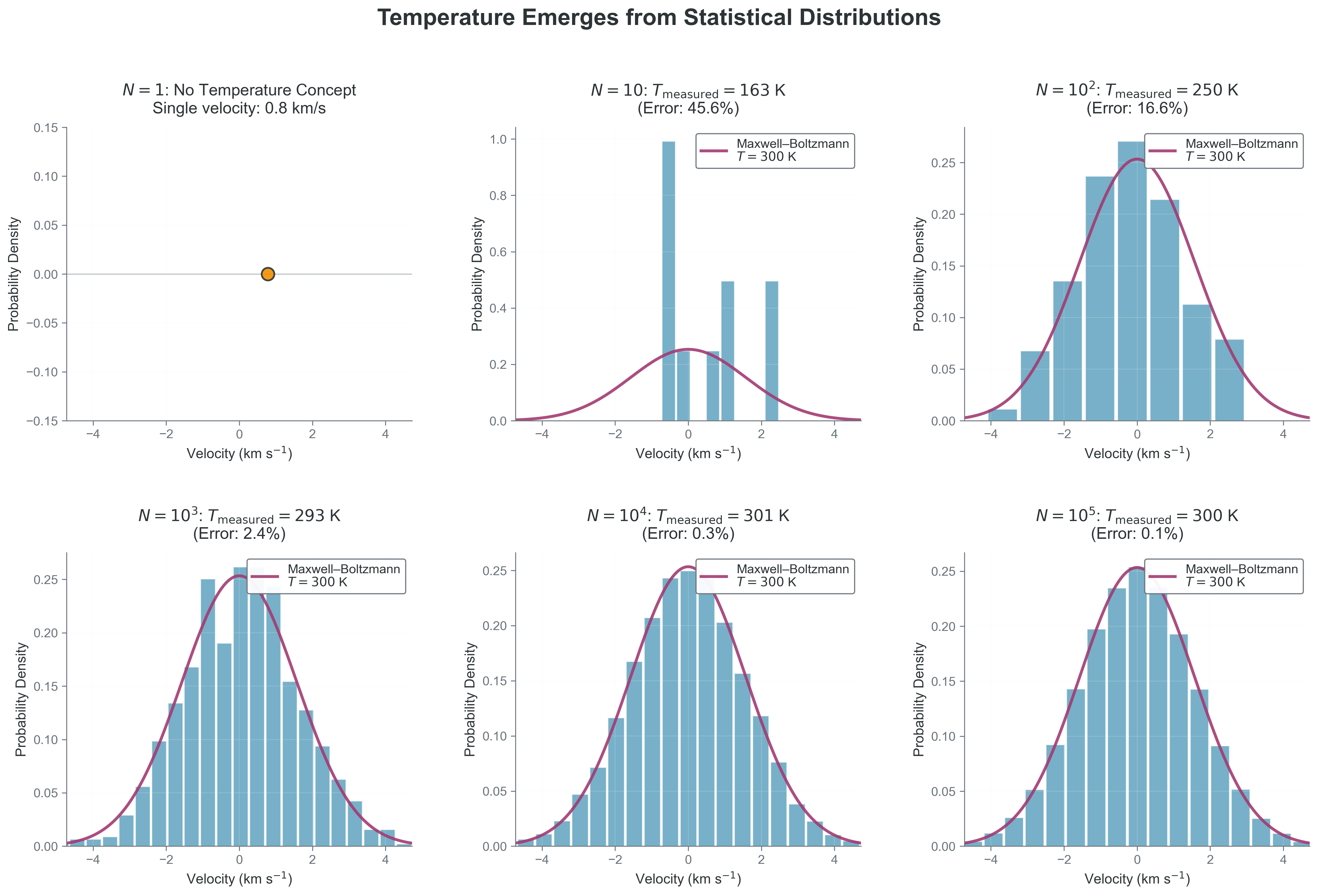— Figure 1:**Temperature emerges as a meaningful statistical concept only with sufficient particles.**
This figure demonstrates the fundamental truth that temperature is not a property of individual particles, but rather a parameter characterizing the width (variance) of velocity distributions across ensembles. For a single particle (N=1), temperature is undefined—we can only specify its individual velocity. As particle number increases through powers of 10 (N = 10, 10², 10³, 10⁴, 10⁵), the measured temperature (calculated from velocity variance using T = m⟨v²⟩/k_B) converges toward the true value of 300 K, with errors decreasing from ~54% (N=10) to ~0.1% (N=10⁵). The histograms progressively match the theoretical Maxwell-Boltzmann distribution (red curves), illustrating how macroscopic thermodynamic properties emerge from microscopic statistical behavior. This statistical foundation underlies all of thermodynamics—from stellar interiors maintaining local thermal equilibrium despite enormous gradients, to neural network “temperature” parameters controlling output distribution spreads in machine learning.

🎯 Connection to Equipartition and LTE

The equipartition theorem — that each quadratic degree of freedom gets $\tfrac{1}{2}k_B T$ of energy — is a consequence of temperature being the distribution parameter, not its definition.

Why this matters for stellar physics: In stellar interiors, where collision times are ~10^-9 seconds, particles constantly exchange energy and maintain their thermal distribution. This is why we can use a single temperature at each point despite enormous gradients — locally, there are always enough particles colliding frequently enough to define and maintain a meaningful temperature.

The universal pattern:

Monatomic gas: 3 translational DOF → $E = \frac{3}{2}Nk_B T$
Diatomic gas: 3 translation + 2 rotation → $E = \frac{5}{2}Nk_B T$ (at room temp)
Solid: 3 kinetic + 3 potential → $E = 3Nk_B T$ (Dulong-Petit law)

Temperature democratically distributes energy — every quadratic degree of freedom gets an equal share, regardless of its physical nature.

This connection appears everywhere:

Neural networks: “Temperature” in softmax controls output distribution spread
MCMC: “Temperature” in simulated annealing controls parameter space exploration
Optimization: High temperature = exploration, low temperature = exploitation

1.2 Pressure Emerges from Chaos¶

Priority: 🔴 Essential

Here’s something remarkable: the steady pressure you feel from the atmosphere emerges from pure chaos. Air molecules hit your skin randomly, from random directions, with random speeds. Yet somehow this randomness produces perfectly steady, predictable pressure. How?

Physical intuition: Think of rain on a roof. Individual drops hit randomly — different spots, different times, different speeds. But you hear steady white noise and the roof feels constant pressure. Gas pressure works the same way — chaos at the microscopic scale averages into order at the macroscopic scale.

Building Pressure from Individual Collisions¶

Let’s derive pressure step by step, starting from single molecular collisions.

Step 1: Single collision momentum transfer When a molecule with velocity $v_x$ hits the wall and bounces back elastically:

Initial momentum toward wall: $p_i = mv_x$
Final momentum away from wall: $p_f = -mv_x$
Momentum transferred to wall: $\Delta p = p_i - p_f = 2mv_x$

Step 2: Collision rate How many molecules hit the wall per second? Consider molecules within distance $v_x \Delta t$ of the wall:

Volume that can reach wall: $A \cdot v_x \Delta t$ (where A is wall area)
Number of molecules in this volume: $n \cdot A \cdot v_x \Delta t$ (where n is number density)
But only half move toward the wall: $\frac{1}{2} n \cdot A \cdot v_x \Delta t$

Step 3: Total momentum transfer per unit time Force = momentum transfer per unit time. For all molecules:

F = \frac{\text{total momentum transfer}}{\Delta t} = \frac{1}{2} n A \cdot 2m \langle v_x^2 \rangle = n A m \langle v_x^2 \rangle

(3)

Here we use the ensemble average $\langle v_x^2 \rangle$ because molecules have different velocities.

Step 4: From force to pressure Pressure is force per unit area:

P = \frac{F}{A} = nm\langle v_x^2 \rangle

(4)

For Maxwell-Boltzmann distributed velocities, $\langle v_x^2 \rangle = k_B T/m$ , giving:

\boxed{P = nk_B T}

(5)

The ideal gas law emerges from pure statistics — no empirical fitting needed!

Visual insight: Random molecular collisions → steady macroscopic pressure through averaging.

Maxwell-Boltzmann molecular chaos averages to create steady macroscopic pressure. This scientifically accurate illustration demonstrates how pressure emerges from statistical mechanics: individual molecular collisions (gray points, sized proportional to momentum transfer) follow Maxwell-Boltzmann velocity statistics and create highly variable momentum transfers. However, their cumulative running average (blue line) converges smoothly to the theoretical pressure value (red dashed line). The particle sizes visually represent the physical reality that some molecules move much faster than others, yet statistical averaging over ~2000 collisions produces the stable pressure we observe macroscopically. This fundamental principle — microscopic chaos → macroscopic order through averaging — underlies all thermodynamic properties from atmospheric pressure to stellar interior conditions. 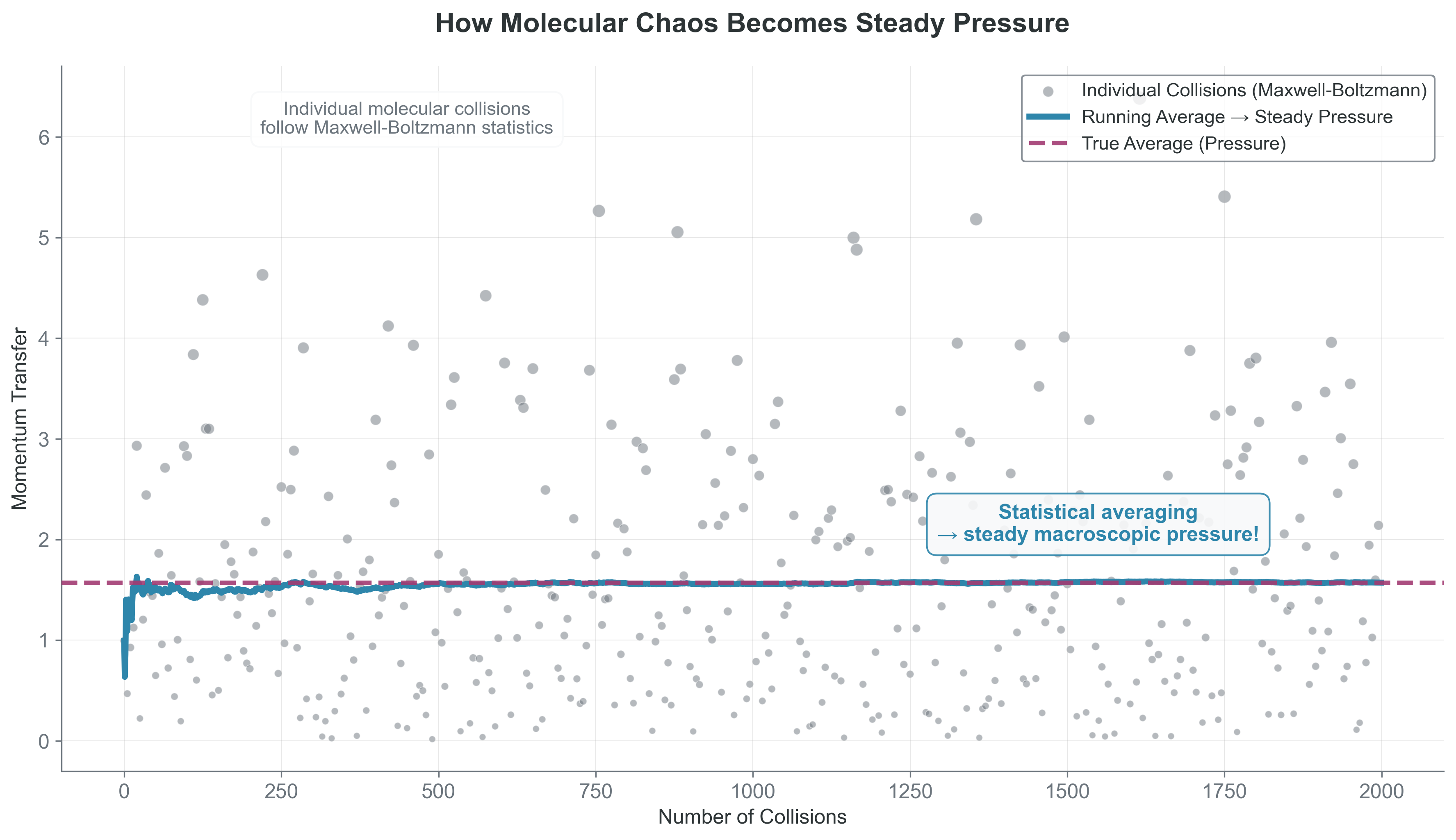— Figure 2:**Maxwell-Boltzmann molecular chaos averages to create steady macroscopic pressure.**
This scientifically accurate illustration demonstrates how pressure emerges from statistical mechanics: individual molecular collisions (gray points, sized proportional to momentum transfer) follow Maxwell-Boltzmann velocity statistics and create highly variable momentum transfers. However, their cumulative running average (blue line) converges smoothly to the theoretical pressure value (red dashed line). The particle sizes visually represent the physical reality that some molecules move much faster than others, yet statistical averaging over ~2000 collisions produces the stable pressure we observe macroscopically. This fundamental principle — microscopic chaos → macroscopic order through averaging — underlies all thermodynamic properties from atmospheric pressure to stellar interior conditions.

The key insight: Macroscopic observables are ensemble averages of microscopic quantities:

Pressure: average momentum transfer
Current: average charge flow
Magnetization: average spin alignment
Neural network output: average over dropout masks

This principle — individual randomness + large numbers = predictable averages — makes both physics and machine learning possible.

1.3 The Central Limit Theorem: Why Everything is Gaussian¶

Priority: 🔴 Essential

In Section 1.2, we saw that averaging chaotic molecular collisions creates steady pressure. But WHY does averaging create such remarkable stability? Why don’t we sometimes feel pressure fluctuations? The answer is one of the most powerful theorems in mathematics: the Central Limit Theorem (CLT).

Why this matters for pressure stability:

Remember from Section 1.2 that pressure is the average of N molecular momentum transfers:

P \propto \frac{1}{N}\sum_{i=1}^N \text{(momentum transfer)}_i

(7)

Each collision transfers random momentum. By the CLT:

For $N = 100$ : pressure fluctuates by ~10%
For $N = 10^6$ : pressure fluctuates by ~0.1%
For $N = 10^{23}$ (real gas): fluctuates by ~10^-11%

The CLT guarantees that pressure becomes incredibly stable as N increases!

Why air pressure doesn’t fluctuate: Each cm³ of air contains ~ $2.5×10¹⁹$ molecules. The relative pressure fluctuations scale as $1/\sqrt{N} \sim 10⁻¹⁰$ , far too small for any measurement to detect. This is why macroscopic properties appear perfectly stable despite microscopic chaos.

💻 Computational Demo: Watch Chaos Become Gaussian

Copy and paste this code to see the Central Limit Theorem in action:

import numpy as np
import matplotlib.pyplot as plt
from scipy import stats

def demonstrate_clt(original_distribution='exponential'):
    """Show how any distribution becomes Gaussian when summed."""
    
    # Choose a decidedly NON-Gaussian starting distribution
    if original_distribution == 'exponential':
        sample_func = lambda size: np.random.exponential(1.0, size)
        dist_name = "Exponential (very skewed!)"
    elif original_distribution == 'uniform':
        sample_func = lambda size: np.random.uniform(-1, 1, size)  
        dist_name = "Uniform (flat!)"
    
    # Show different levels of summing
    sum_sizes = [1, 5, 20, 100]  # how many to add together
    fig, axes = plt.subplots(2, 2, figsize=(10, 8))
    
    for i, n_sum in enumerate(sum_sizes):
        ax = axes[i//2, i%2]
        
        # Create sums of n_sum random variables
        sums = []
        for _ in range(5000):  # 5000 trials
            sample = sample_func(n_sum)  # draw n_sum random numbers
            sums.append(np.sum(sample))  # sum them up
        
        # Standardize: mean=0, variance=1
        sums = np.array(sums)
        mean_theory = n_sum * 1.0  # theoretical mean
        std_theory = np.sqrt(n_sum) * 1.0  # theoretical std
        sums_std = (sums - mean_theory) / std_theory
        
        # Plot histogram
        ax.hist(sums_std, bins=30, density=True, alpha=0.7, 
               color='skyblue', edgecolor='black')
        
        # Overlay perfect Gaussian
        x = np.linspace(-4, 4, 200)
        ax.plot(x, stats.norm.pdf(x), 'r-', linewidth=2, 
               label='Perfect Gaussian')
        
        # Titles showing the magic
        if n_sum == 1:
            ax.set_title(f'{dist_name}\n(Original - not Gaussian!)')
        else:
            ax.set_title(f'Sum of {n_sum} variables\n(Getting Gaussian!)')
        
        ax.set_xlim(-4, 4)
        ax.set_ylim(0, 0.45)
        ax.legend()
        ax.grid(True, alpha=0.3)
    
    plt.suptitle('Central Limit Theorem: Any Distribution → Gaussian', fontsize=14)
    plt.tight_layout()
    plt.show()
    
    print("🎯 The Magic: No matter how weird your starting distribution,")
    print("   sums ALWAYS become Gaussian! This is why Gaussians are everywhere.")

# Try it with different starting distributions!
demonstrate_clt('exponential')  # Very skewed → Gaussian
# demonstrate_clt('uniform')      # Flat → Gaussian

Try changing the starting distribution - the CLT works for ANY distribution with finite variance!

The Central Limit Theorem transforms any distribution into a Gaussian through summation. This figure demonstrates the remarkable universality of the CLT by starting with exponential distributions (highly skewed, far from Gaussian) and showing their progressive transformation into perfect Gaussian distributions as we sum increasing numbers of variables. The panels show sums of N = 1,5,20,100,500,2000 exponential random variables, each standardized to have mean=0 and variance=1. As N increases, the distributions (blue histograms) converge remarkably toward the theoretical Gaussian curve (red line), with perfect agreement achieved by N=500. This universality explains why Gaussian distributions appear throughout physics — from measurement errors (sums of many small random errors) to stellar velocities (sums of gravitational interactions) to neural network initialization (sums of many small weight updates). The CLT is fundamental to why macroscopic physics is predictable despite microscopic chaos. 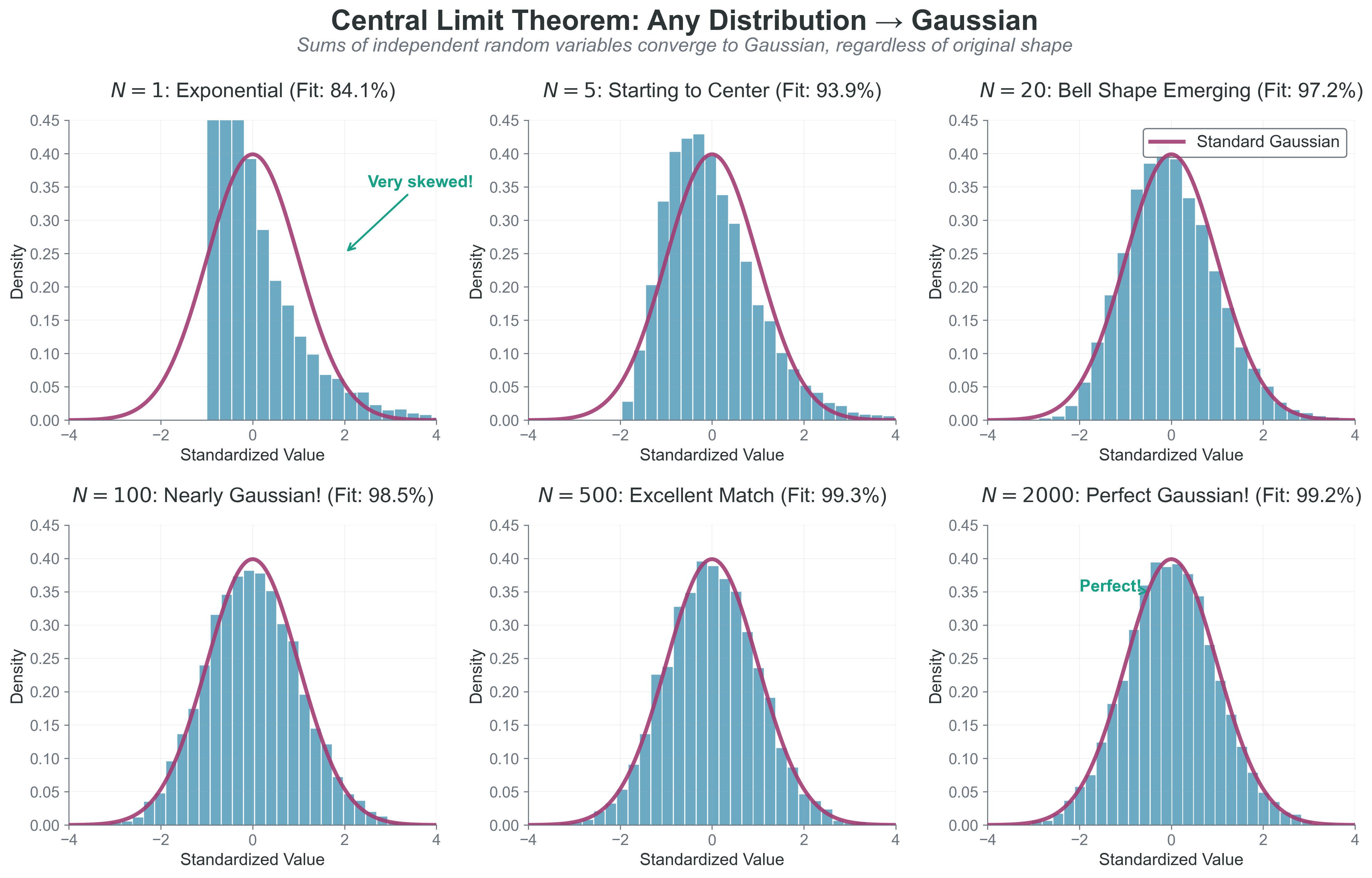— Figure 3:**The Central Limit Theorem transforms any distribution into a Gaussian through summation.** This figure demonstrates the remarkable universality of the CLT by starting with exponential distributions (highly skewed, far from Gaussian) and showing their progressive transformation into perfect Gaussian distributions as we sum increasing numbers of variables. The panels show sums of $N = 1,5,20,100,500,2000$ exponential random variables, each standardized to have mean=0 and variance=1. As N increases, the distributions (blue histograms) converge remarkably toward the theoretical Gaussian curve (red line), with perfect agreement achieved by N=500. This universality explains why Gaussian distributions appear throughout physics — from measurement errors (sums of many small random errors) to stellar velocities (sums of gravitational interactions) to neural network initialization (sums of many small weight updates). The CLT is fundamental to why macroscopic physics is predictable despite microscopic chaos.

Example: Velocity of a dust grain A dust grain in air gets hit by ~10¹⁰ molecules per second. Each collision imparts a random momentum kick. By CLT:

Individual kicks: random, unpredictable
Sum of kicks: Gaussian distribution
Result: Brownian motion with Gaussian velocity distribution
This is why Einstein could use Brownian motion to prove atoms exist!

This is why we see Gaussians everywhere:

Measurement errors: sum of many small random errors
Stellar velocities: sum of many gravitational interactions
Neural network weights: initialized as Gaussian (sum of many small updates)

The profound implication: We don’t need to know the details of individual interactions. The CLT guarantees that collective behavior will be Gaussian, making physics predictable despite underlying chaos.

1.4 The Maximum Entropy Principle¶

Priority: 🔴 Essential

🌟 The More You Know: Boltzmann’s Tragic Story and Ultimate Vindication

Ludwig Boltzmann (1844-1906) gave us the statistical foundation of thermodynamics, but he paid a terrible price. His equation S = k log W, linking entropy to the number of microscopic states, is so fundamental it’s carved on his tombstone in Vienna.

Boltzmann spent his career arguing that atoms were real and that thermodynamics emerged from their statistical behavior. This seems obvious now, but in the late 1800s, many prominent physicists believed atoms were just a convenient fiction. Ernst Mach and Wilhelm Ostwald led fierce attacks on Boltzmann’s ideas, arguing that science should only deal with directly observable quantities.

The constant criticism took its toll. Boltzmann suffered from what we’d now recognize as severe depression and possibly bipolar disorder. He called his depressive episodes “my terrible enemy” and his manic periods “my good friend.” The academic battles worsened his condition.

In September 1906, while on vacation with his family in Trieste, Boltzmann took his own life. He was 62. His daughter found him.

The tragedy deepens: Boltzmann died just before his vindication. In 1905, Einstein’s paper on Brownian motion provided observable proof of atoms. By 1908, experiments by Jean Perrin confirmed atomic theory beyond doubt. Within a few years of Boltzmann’s death, everyone accepted that he had been right all along.

Today, Boltzmann’s constant $k$ appears in nearly every equation in this module. The maximum entropy principle he pioneered underlies everything from black hole thermodynamics to machine learning. When you write $e^{(-E/kT)}$ , you’re using Boltzmann’s revolutionary insight that probability and energy are linked through exponentials.

His story reminds us that being right isn’t always enough in science — timing and community acceptance matter too. It also reminds us that the giants whose equations we casually manipulate were human beings who struggled, doubted, and sometimes broke under the pressure of their brilliance.

You have a container of gas. You can measure its average energy, but you can’t track 10²³ individual molecules. What velocity distribution should you assume? This question leads to one of the most profound principles in physics: maximum entropy.

The inference problem: Imagine you know only that the average molecular energy is $E_0$ . You must guess the full distribution of energies. What’s the most honest guess?

Option 1: Assume all molecules have energy $E_0$

Very specific — claims all molecules are identical
Extremely unlikely (why would they all be the same?)
Makes strong claims with no justification

Option 2: Assume most molecules are near $E_0$ with small spread

Less specific but still assumes a particular pattern
Where did you get the specific spread from?
Still making unjustified assumptions

Option 3: Assume the broadest (maximum entropy) distribution consistent with average $E_0$

Makes the fewest assumptions
Admits maximum ignorance about what you don’t know
Doesn’t invent patterns that might not exist

Maximum entropy is intellectual honesty in mathematical form.

🎯 Why This Matters: What “Least Biased” Really Means

When we say “least biased” or “maximum entropy,” we mean: “I will admit my ignorance about everything I don’t actually know.”

The Procedure:

List what you actually know (constraints)
Find the probability distribution that:
- Satisfies your constraints
- Has maximum uncertainty (entropy) about everything else
This distribution makes no claims beyond your actual knowledge

Why Nature Uses It:

Collisions randomize velocities → maximum entropy given energy
Light scattering randomizes photons → blackbody spectrum
Heat flow randomizes energy → thermal equilibrium

In Machine Learning:

Don’t know class probabilities? Use uniform prior (max entropy with no constraints)
Know only mean and variance? Use Gaussian (max entropy with those constraints)
Softmax is literally the max entropy distribution for classification

What is entropy? Entropy measures uncertainty in a distribution:

S = -k_B \sum_i p_i \ln p_i

(8)

All outcomes equally likely → maximum entropy
One outcome certain → zero entropy
More spread → higher entropy

📝 Mathematical Deep Dive: Maximum Entropy as Optimization

The Optimization Problem:

Maximize: $S = -\sum_i p_i \ln p_i$ (entropy)

Subject to:

Normalization: $\sum_i p_i = 1$ (probabilities sum to 1)
Energy constraint: $\sum_i p_i E_i = E_0$ (average energy is fixed)

Solution via Lagrange Multipliers:

Form the Lagrangian:

\mathcal{L} = -\sum_i p_i \ln p_i - \alpha\left(\sum_i p_i - 1\right) - \beta\left(\sum_i p_i E_i - E_0\right)

(9)

Taking derivatives and solving gives:

\boxed{p_j = \frac{e^{-\beta E_j}}{Z}}

(10)

where $Z = \sum_j e^{-\beta E_j}$ is the partition function (normalization constant).

This is the Boltzmann distribution! We identify $\beta = 1/k_B T$ , so temperature is literally the Lagrange multiplier enforcing the energy constraint.

Connection to Machine Learning:

This is EXACTLY how constrained optimization works in ML:

System	Objective	Constraint	Lagrange Multiplier
Statistical mechanics	Maximize entropy	Fixed energy	Temperature (1/kT)
Neural network	Minimize loss	Weight penalty	Regularization λ
Variational Autoencoder	Minimize reconstruction	KL divergence	β parameter

The same optimization framework appears everywhere!

Maximum Entropy Principle explains why stellar atmospheres follow Maxwell-Boltzmann distributions. Left: If all particles had identical energy (biased assumption), entropy = 0. Center: Given only the constraint of fixed mean energy, the exponential distribution maximizes entropy (S = 1 + ln(kT) ≈ 2.10), representing nature’s least biased choice. Right: In stellar atmospheres, this manifests as exponential decay in energy level populations following the Boltzmann law: n/n₀ = exp(-E/kT), which determines spectral line ratios and ionization fractions. 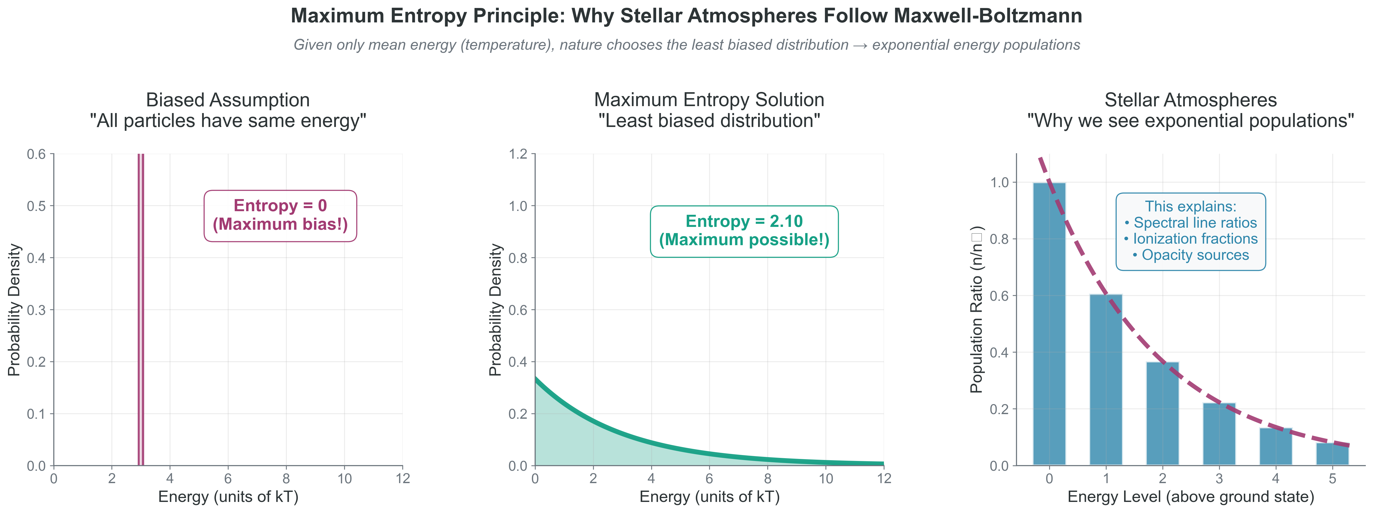— Figure 4:**Maximum Entropy Principle explains why stellar atmospheres follow Maxwell-Boltzmann distributions.** Left: If all particles had identical energy (biased assumption), entropy = 0. Center: Given only the constraint of fixed mean energy, the exponential distribution maximizes entropy (S = 1 + ln(kT) ≈ 2.10), representing nature’s least biased choice. Right: In stellar atmospheres, this manifests as exponential decay in energy level populations following the Boltzmann law: n/n₀ = exp(-E/kT), which determines spectral line ratios and ionization fractions.

💻 Try This: Generate Maximum Entropy Distributions

Copy this code to explore different constraints and see what distributions emerge:

import numpy as np
from scipy import stats

def max_entropy_demo(constraint='mean_only'):
    """Show what maximum entropy gives under different constraints."""
    
    if constraint == 'mean_only':
        # Only know mean energy = 3 units
        mean_E = 3.0
        dist = stats.expon(scale=mean_E)  # Exponential: max entropy given mean
        print(f"Constraint: Mean energy = {mean_E}")
        print(f"Max entropy solution: Exponential with scale={mean_E}")
        print(f"Entropy = {dist.entropy():.2f} nats")
        
    elif constraint == 'mean_and_variance':
        # Know mean and variance  
        mean_E = 3.0
        var_E = 2.0
        dist = stats.norm(mean_E, np.sqrt(var_E))  # Gaussian: max entropy given mean & var
        print(f"Constraints: Mean = {mean_E}, Variance = {var_E}")
        print(f"Max entropy solution: Gaussian")
        print(f"Entropy = {dist.entropy():.2f} nats")
        
    return dist

# Try different constraints
print("🎯 What does maximum entropy give?")
print("=" * 40)
exp_dist = max_entropy_demo('mean_only')
print()
gauss_dist = max_entropy_demo('mean_and_variance')

The insight: Maximum entropy automatically chooses the “right” distribution based on what you actually know!

Why this matters everywhere:

Field	Maximum Entropy Application
Physics	Boltzmann distribution for particles
Information Theory	Optimal compression and coding
Machine Learning	Softmax for classification
Bayesian Inference	Least informative priors
Image Processing	Deblurring and reconstruction

The deep connection: The softmax function in neural networks IS the Boltzmann distribution:

p(class_i) = \frac{e^{z_i/T}}{\sum_j e^{z_j/T}}

(11)

Same math, different labels. Temperature controls exploration vs exploitation in both physics and ML.

Bridge to Part 2: Now that you understand how macroscopic properties emerge from distributions (temperature from velocity spread, pressure from averaging, Gaussians from CLT, and exponentials from maximum entropy), Part 2 will give you the mathematical tools to manipulate these distributions for practical calculations.