Statistical Thinking Foundations

COMP 536 | Week 6 Statistical Thinking Foundations

Dr. Anna Rosen

2026-04-22

Learning Outcomes

By the end of this lecture, you will be able to:

  • Explain why temperature and pressure are ensemble-level statistical quantities
  • Apply CLT, marginalization, and ergodicity ideas to computational diagnostics
  • Use moments to connect physical interpretation to machine-learning practice
  • Choose and validate sampling strategies for Project 2 and Project 3 workflows
  • Build a trustworthy stochastic computation with reproducibility and diagnostics

Why This Lecture Exists

You are about to use Monte Carlo methods, random sampling, and population modeling throughout COMP 536.

Without statistical foundations, those methods become recipes without understanding.

With strong foundations, you can diagnose when a method is failing and fix it quickly.

Roadmap (65 Minutes)

Concept Loops

  • Loop A: Emergence (temperature, pressure, CLT)
  • Loop B: Core statistical tools (correlation, marginalization, uncertainty)
  • Loop C: Moments as information compression
  • Loop D: Sampling for realistic simulation

Practice Components

  • Livecoding-lite with deterministic snippets
  • Code Craft micro-segment
  • Exit Ticket for transfer to Projects 2 and 3

Loop A: Emergence from Randomness

Predict: Can One Particle Have a Temperature?

A single particle has velocity and kinetic energy.

Does it have a temperature?

    1. Yes, because kinetic energy implies temperature
    1. No, because temperature describes a distribution over many particles

Reveal: Temperature is a Distribution Parameter

Temperature scales with velocity variance across an ensemble, not with one particle state.

Play: Estimate Temperature from Velocity Samples

Purpose: infer an ensemble temperature proxy from sampled velocities. Inputs/Outputs: input n_samples; output sample variance and inferred relative temperature. Pitfall: interpreting small-N fluctuation as a physics change rather than sampling noise.

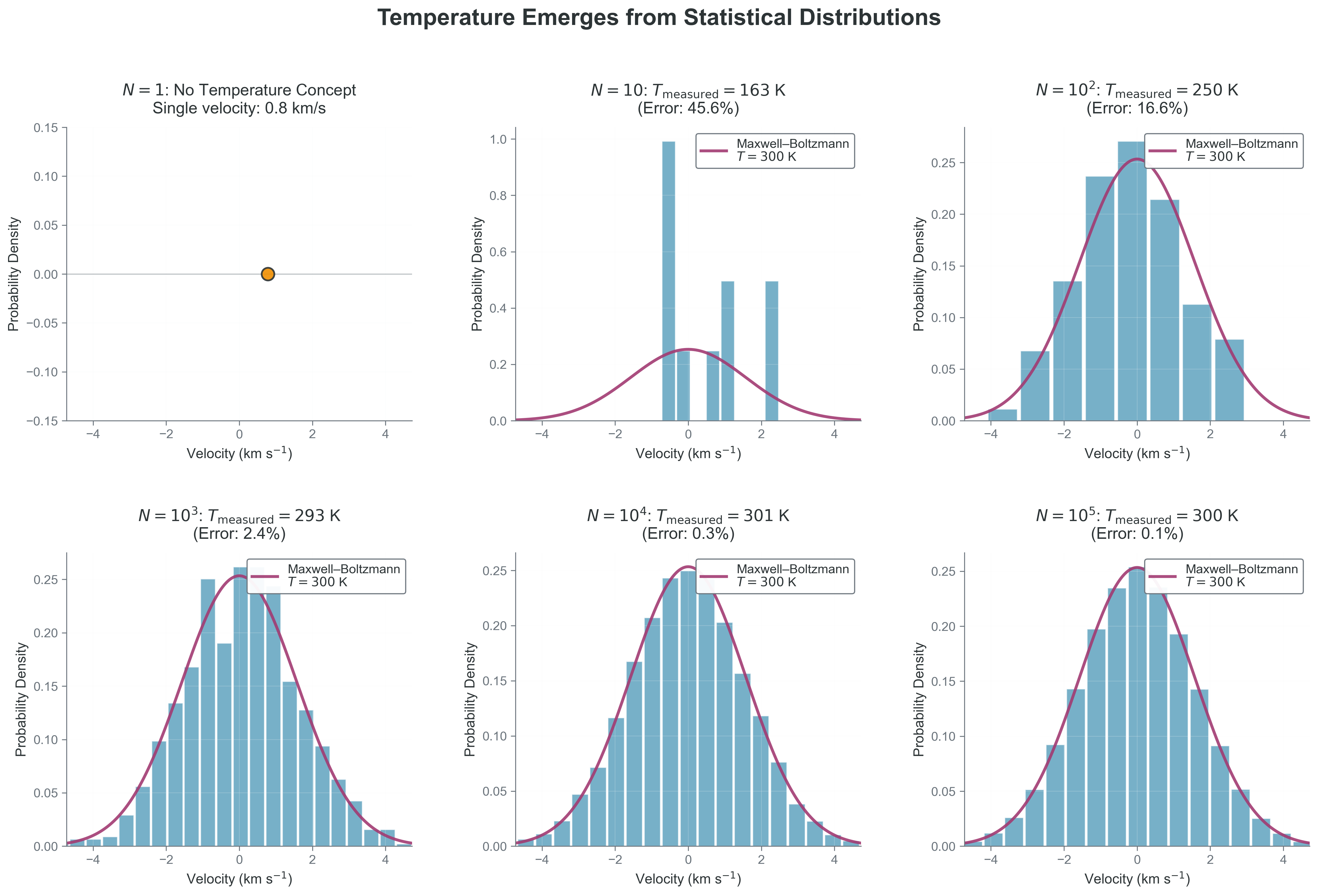
def infer_temperature_proxy(n_samples, sigma_true=1.0):
    v = rng.normal(0.0, sigma_true, n_samples)
    variance = np.var(v, ddof=1)
    return variance

for n in [20, 200, 2000, 20000]:
    var_hat = infer_temperature_proxy(n)
    print(f"N={n:5d}  variance~{var_hat:0.4f}")

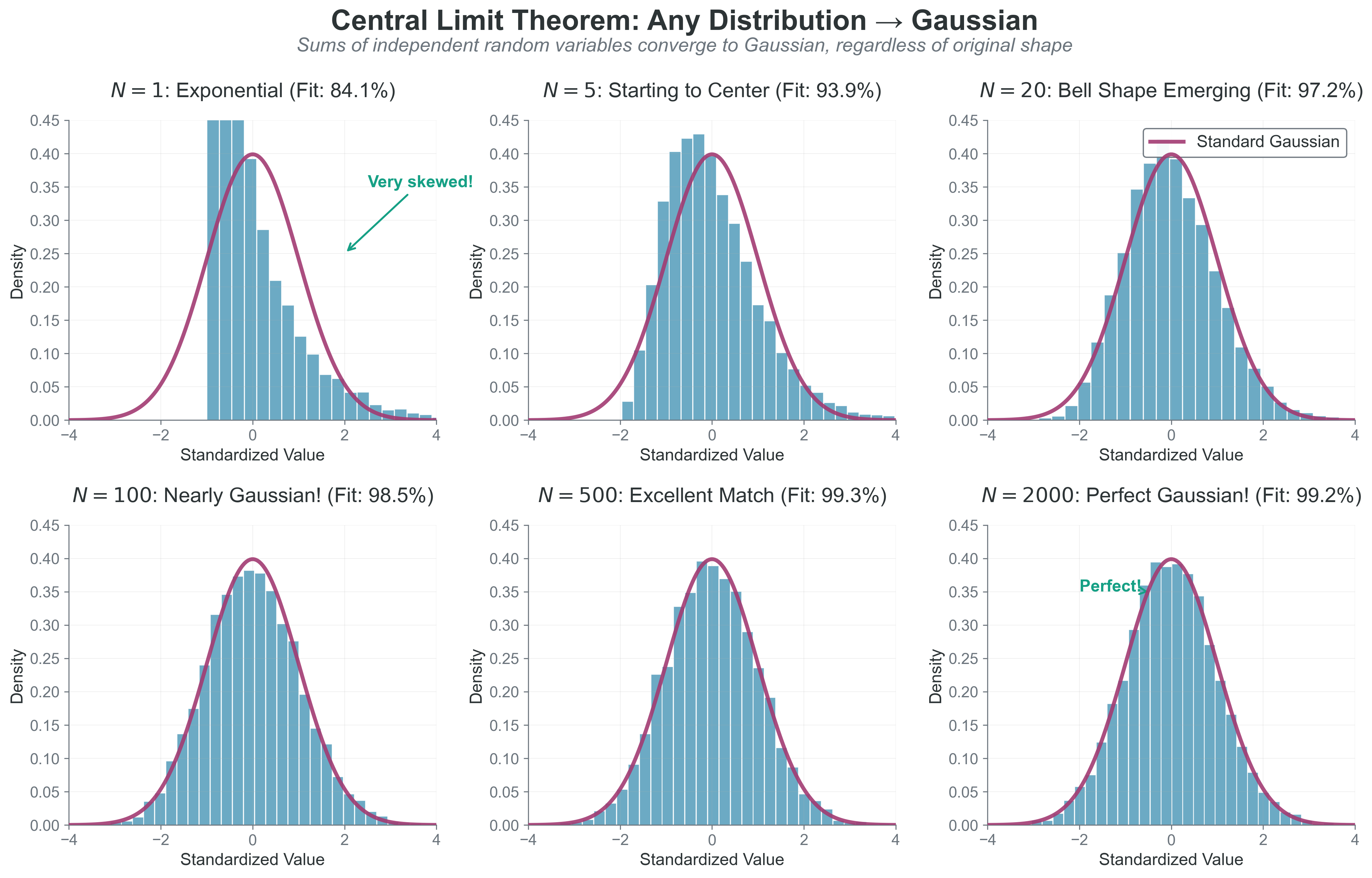
print("Interpretation: larger N gives a more stable estimate of ensemble properties.")
N=   20  variance~1.1810
N=  200  variance~0.8353
N= 2000  variance~0.9754
N=20000  variance~1.0213
Interpretation: larger N gives a more stable estimate of ensemble properties.

Explain: Why Pressure is Stable

CLT explains why aggregate collision statistics approach Gaussian behavior and stabilize macroscopic pressure.

Loop A: Predict - Play - Explain Checkpoint

  • Predict: if particle count increases by \(100\times\), what happens to relative fluctuation scale?
  • Play: compare sample means for \(N=10^2\) and \(N=10^4\) draws from the same parent distribution.
  • Explain: use the \(1/\sqrt{N}\) law to justify whether a mismatch is expected.

Loop B: Tools for Inference and Diagnostics

Correlation is Not Independence

Uncorrelated can still be dependent, and dependence structure controls uncertainty propagation.

Marginalization: Keep What You Can Observe

From 3D velocity density to speed density:

\[g(v) = 4\pi v^2 f_{\vec{v}}(v)\]

This is where geometry enters through the \(v^2\) shell factor.

Error Propagation and Convergence Rates

Statistical uncertainty propagates predictably, and Monte Carlo precision improves as \(1/\sqrt{N}\).

Play: Monte Carlo Error Scaling in Practice

Purpose: quantify how estimate precision improves with sample count. Inputs/Outputs: inputs draw counts N; outputs mean estimate and standard error. Pitfall: expecting linear error reduction with compute budget.

def mc_estimate_and_stderr(n):
    x = rng.normal(0.0, 1.0, n)
    mean = np.mean(x)
    stderr = np.std(x, ddof=1) / np.sqrt(n)
    return mean, stderr

for n in [10**2, 10**3, 10**4, 10**5]:
    mean, se = mc_estimate_and_stderr(n)
    print(f"N={n:6d}  mean={mean:+0.4f}  stderr={se:0.4f}")
N=   100  mean=-0.1450  stderr=0.0999
N=  1000  mean=-0.0130  stderr=0.0309
N= 10000  mean=+0.0010  stderr=0.0101
N=100000  mean=+0.0057  stderr=0.0032

Loop B: Predict - Play - Explain Checkpoint

  • Predict: if covariance is ignored, are propagated uncertainties usually under- or over-estimated?
  • Play: recompute one estimate with correlated vs uncorrelated assumptions.
  • Explain: decide whether mismatch came from dependence structure, wrong propagation assumptions, or finite sample count.

Loop C: Moments as Information Compression

Moments: What They Preserve and What They Lose

For a distribution \(f(x)\):

\[M_n = E[X^n]\]

Low-order moments often capture core behavior for smooth unimodal distributions, but can miss multimodality and heavy tails.

Physics and ML Use the Same Statistical Machinery

  • Physics: variance links to velocity dispersion and thermal width.
  • ML: first/second moments appear in momentum and adaptive optimizers.
  • Shared move: compress high-dimensional stochastic behavior into stable summary statistics.

Play: Moment Tracking in a Synthetic Stream

Purpose: observe how mean/variance/skewness evolve as sample size grows. Inputs/Outputs: input sample stream; output running first three moments. Pitfall: over-interpreting unstable skewness at low sample count.

from scipy.stats import skew

samples = rng.normal(loc=0.0, scale=1.0, size=5000)
for n in [50, 200, 1000, 5000]:
    x = samples[:n]
    m1 = np.mean(x)
    m2 = np.var(x, ddof=1)
    m3 = skew(x, bias=False)
    print(f"N={n:4d}  mean={m1:+0.3f}  var={m2:0.3f}  skew={m3:+0.3f}")
N=  50  mean=+0.180  var=0.473  skew=-0.258
N= 200  mean=-0.019  var=0.803  skew=-0.126
N=1000  mean=-0.045  var=0.992  skew=-0.017
N=5000  mean=-0.004  var=1.015  skew=-0.002

Loop C: Predict - Play - Explain Checkpoint

  • Predict: which moment stabilizes slowest for symmetric noise, variance or skewness?
  • Play: compare stabilization rates across \(N\).
  • Explain: connect sensitivity to rare events and tail sampling.

Loop D: Sampling to Build Simulations

Inverse Transform and Rejection Sampling

Inverse transform is exact when \(F^{-1}\) is tractable; rejection sampling is flexible when it is not.

Power Laws and Astrophysical Populations

For \(f(m) \propto m^{-\alpha}\) on \([m_{\min}, m_{\max}]\), careful inversion gives physically realistic mass draws.

Isotropic 3D Sampling Matters

Use - \(\mu = \cos\theta \sim U(-1,1)\) - \(\phi \sim U(0,2\pi)\) - \(\theta = \arccos(\mu)\)

to avoid pole clustering artifacts.

Play: Minimal Isotropic Direction Sampler

Purpose: generate unbiased direction vectors for 3D initial conditions. Inputs/Outputs: input n; output arrays (x, y, z) on the unit sphere. Pitfall: sampling \(\theta\) uniformly in \([0,\pi]\) creates non-isotropic clustering.

def sample_isotropic_directions(n):
    mu = rng.uniform(-1.0, 1.0, n)
    phi = rng.uniform(0.0, 2 * np.pi, n)
    theta = np.arccos(mu)

    x = np.sin(theta) * np.cos(phi)
    y = np.sin(theta) * np.sin(phi)
    z = np.cos(theta)
    return x, y, z

x, y, z = sample_isotropic_directions(5)
print(np.round(np.column_stack([x, y, z]), 3))
[[ 0.625  0.718 -0.306]
 [-0.33   0.769  0.548]
 [ 0.406  0.911  0.079]
 [-0.472  0.514 -0.716]
 [-0.698  0.092  0.71 ]]

Loop D: Predict - Play - Explain Checkpoint

  • Predict: does Monte Carlo error always decrease faster than model bias as compute increases?
  • Play: compare diagnostics for \(10^2\), \(10^4\), \(10^6\) samples.
  • Explain: identify whether failure is geometric bias, model mismatch, or finite-sample noise.

Code Craft: Trustworthy Stochastic Computing

Code Craft Pattern: From Idea to Reliable Result

A reliable stochastic workflow has five explicit steps:

  1. State assumptions and target observable.
  2. Seed randomness for reproducibility.
  3. Validate against analytical or limiting-case checks.
  4. Track uncertainty and convergence rate.
  5. Record diagnostics before interpretation.

Code Craft Example: Reproducible Monte Carlo Estimate

Purpose: demonstrate a reproducible estimate with an explicit uncertainty report. Inputs/Outputs: input n; output estimate and standard error. Pitfall: reporting a point estimate without uncertainty or reproducibility metadata.

def mc_mean_with_error(n, seed=536):
    local_rng = np.random.default_rng(seed)
    draws = local_rng.normal(0.0, 1.0, n)
    estimate = np.mean(draws)
    stderr = np.std(draws, ddof=1) / np.sqrt(n)
    return estimate, stderr

est, se = mc_mean_with_error(20000)
print(f"estimate={est:+0.4f}, stderr={se:0.4f}")
print("Report both estimate and uncertainty in all project summaries.")
estimate=-0.0041, stderr=0.0071
Report both estimate and uncertainty in all project summaries.

Livecoding-lite Fallback Plan

If a live snippet fails during class:

  • Use pre-rendered figures already in the deck.
  • Ask students to predict the expected trend before revealing fallback output.
  • Debrief what the snippet was intended to test.

This keeps pedagogy intact even when runtime is imperfect.

Exit Ticket

Exit Ticket 1: Concept Transfer

You doubled your Monte Carlo sample count from \(N=10^4\) to \(N=4\\times 10^4\).

What should happen to sampling error if everything else is unchanged?

    1. It should drop by about \(2\\times\)
    1. It should drop by about \(4\\times\)
    1. It should stay about the same

Exit Ticket 2: Implementation Decision

For Project 2 initial conditions, you need masses from a power law and isotropic positions.

Which pipeline is most defensible?

  1. Draw \(m\) from an inverse-CDF sampler, then sample directions with \(\mu = \cos\theta \sim U(-1,1)\).
  2. Draw \(\theta \sim U(0,\pi)\) and \(\phi \sim U(0,2\pi)\) directly, then adjust by hand.
  3. Use rejection sampling everywhere without diagnostics.

Write one sentence justifying your choice with one diagnostic you would run.