Part 2: Building Better Methods - Runge-Kutta
Module 3: ODE Methods & Conservation | ASTR 596
Learning Outcomes
By the end of this section, you will be able to:
Derive RK2 and RK4 from multivariate Taylor expansions
Connect RK weights to quadrature rules from Module 2
Implement adaptive timestep control
Analyze when higher-order methods help vs harm
Choose appropriate RK methods based on problem requirements
The Key Insight: Sample Multiple Points
Euler’s fatal flaw is assuming the derivative stays constant over the entire timestep. Real functions curve. Runge-Kutta methods evaluate the derivative at carefully chosen intermediate points, then combine these samples with specific weights to achieve higher-order accuracy.
This is exactly the same principle as quadrature from Module 2! We’re essentially performing numerical integration on:
But now the integrand depends on the unknown solution itself, requiring us to estimate intermediate values.
RK2 - The Midpoint Method
Geometric Intuition
Instead of blindly following the tangent from the starting point, we:
Take a half-step using the initial derivative
Evaluate the derivative at this midpoint
Use this midpoint derivative for the full step
This is analogous to the midpoint rule for integration, which we know from Module 2 is second-order accurate!
Complete Mathematical Formulation
The RK2 midpoint method is a predictor-corrector method:
Stage 1 - Predictor:
Stage 2 - Corrector:
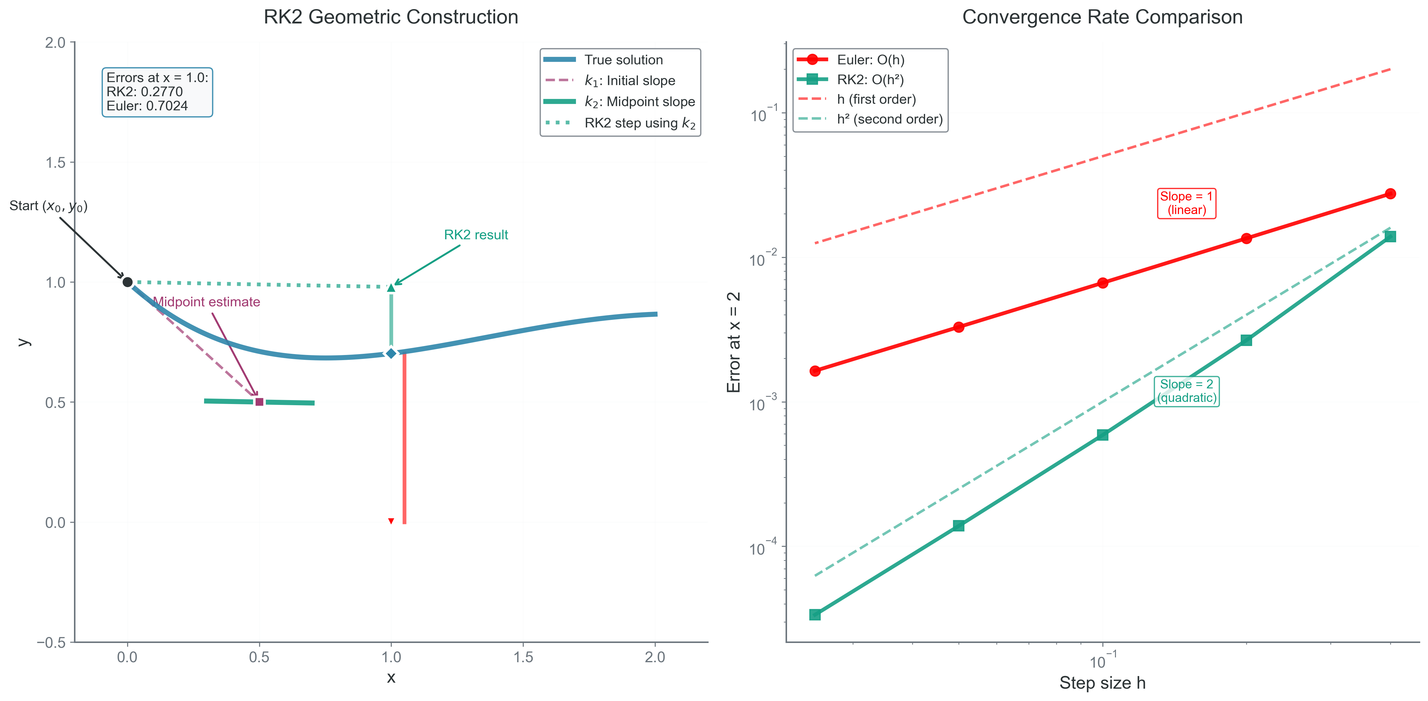
Figure 1:RK2 midpoint method: First evaluate derivative at start (k₁), use it to estimate midpoint, evaluate derivative there (k₂), then use midpoint derivative for full step. This captures solution curvature much better than Euler’s single-point sampling, achieving O(h²) global accuracy. The midpoint derivative (green) provides a better approximation to the average slope over the interval than the initial derivative alone.
Error Analysis via Taylor Series
Using multivariate Taylor expansion, the midpoint derivative becomes:
The RK2 update matches the true solution through :
Local truncation error:
Global error:
RK2 is second-order accurate — halving the timestep reduces error by a factor of 4.
Implementation
def rk2_step(x, t, h, f):
    """Single RK2 (midpoint) step"""
    k1 = f(x, t)

    # Predictor to midpoint
    x_mid = x + 0.5 * h * k1
    t_mid = t + 0.5 * h

    # Evaluate at midpoint
    k2 = f(x_mid, t_mid)

    # Full step using midpoint derivative
    return x + h * k2
RK4 - The Classical Workhorse
RK4 samples the derivative at four carefully chosen points:
Stage 1: (derivative at start)
Stage 2: (derivative at midpoint using )
Stage 3: (derivative at midpoint using )
Stage 4: (derivative at endpoint using )
Final update:
The Connection to Simpson’s Rule
The weights are precisely Simpson’s rule weights from Module 2! This is not a coincidence:
Euler = Rectangle rule: Sample at left endpoint only
RK2 = Midpoint rule: Sample at center
RK4 = Simpson’s rule: Weighted average with parabolic fit
RK4 is essentially applying Simpson’s quadrature to the integral , but with the complication that we must estimate at intermediate points.
Error Analysis
Through Taylor series expansion to fourth order:
Local truncation error:
Global error:
This means halving the timestep reduces error by a factor of 16!
The General Runge-Kutta Framework
All explicit RK methods follow this pattern:
The coefficients define the method and are displayed in a Butcher tableau:
c₁ |
c₂ | a₂₁
c₃ | a₃₁ a₃₂
⋮  | ⋮
cₛ | aₛ₁ aₛ₂ ... aₛ,ₛ₋₁
---|--------------------
   | b₁  b₂  ...  bₛ
For RK4:
0   |
1/2 | 1/2
1/2 | 0   1/2
1   | 0   0   1
----|----------------
    | 1/6 2/6 2/6 1/6
Adaptive Timestep Control
Real problems have varying timescales. When a planet is far from the sun, we can take large steps. During close encounters, we need tiny steps. Adaptive methods adjust dynamically.
The Embedded Runge-Kutta Approach
The idea: compute two different order estimates using the same function evaluations, then use their difference to estimate error.
Runge-Kutta-Fehlberg Method (RK45)
RK45 computes both 4th and 5th order solutions:
Compute six values (shared between both estimates)
Combine with 4th-order weights →
Combine with 5th-order weights →
Error estimate:
Optimal timestep:
If error is acceptable, accept the step and continue. Otherwise, reject and retry with smaller .
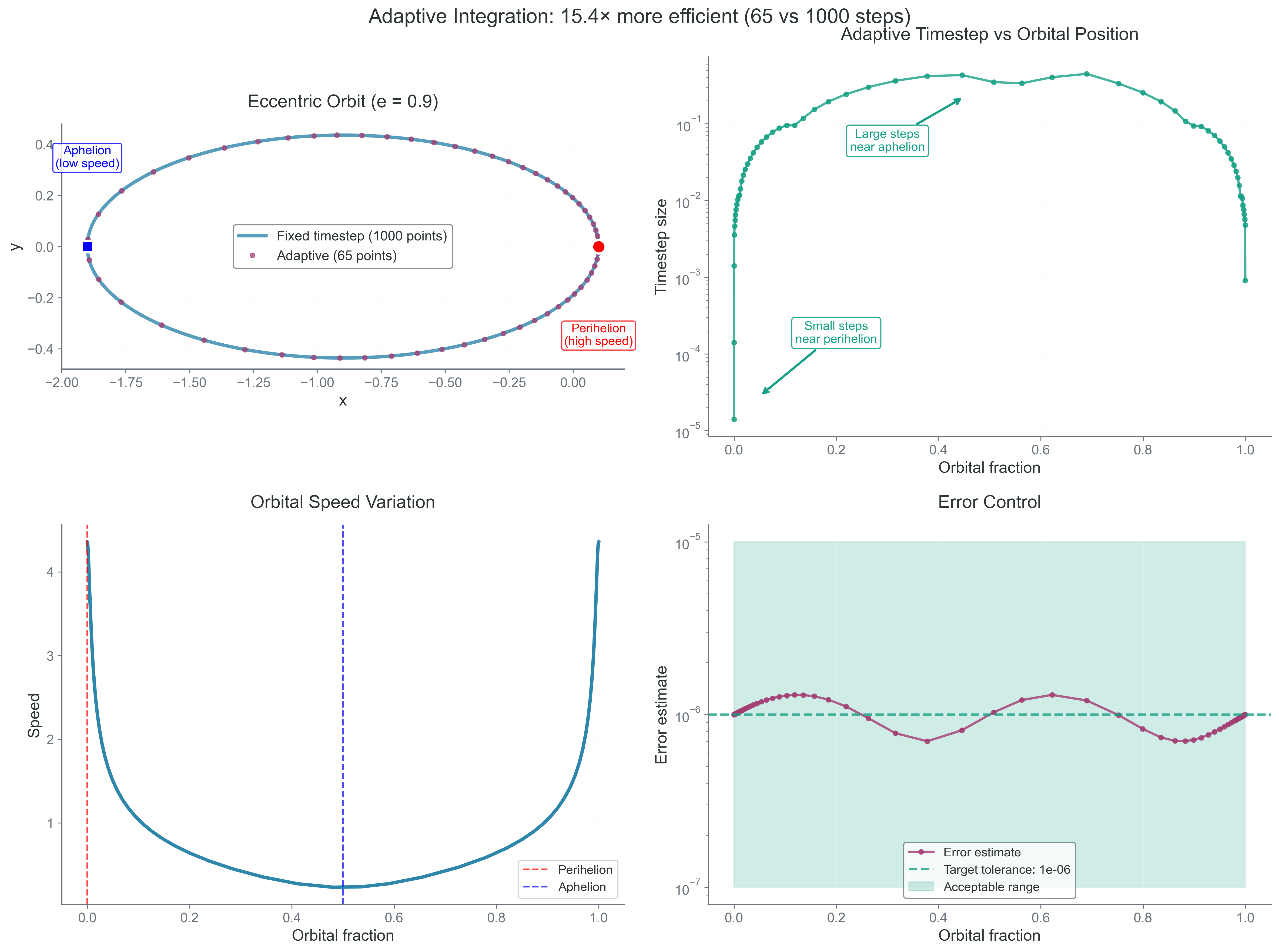
Figure 2:Adaptive timestep control for eccentric orbit (e=0.9). Small steps near perihelion where velocity is high, large steps near aphelion where motion is slow. The top panel shows the elliptical orbit with color-coded timestep sizes, while the bottom panel shows how the timestep varies continuously around the orbit. This concentrates computational effort where dynamics are fastest while maintaining constant error throughout.
When to Use Adaptive Methods
Good for:
Problems with varying timescales
Unknown dynamics
Achieving specified accuracy efficiently
Initial exploration of new systems
Bad for:
Long-term Hamiltonian systems (destroys symplecticity)
Problems requiring uniform time grid
Parallel simulations (variable timesteps complicate synchronization)
Performance Comparison
Let’s compare methods on the Kepler problem (elliptical orbit with ):
| Method | Order | Steps/Orbit | Energy Error After 100 Orbits | CPU Time |
|---|---|---|---|---|
| Euler | 1 | 1000 | +10% | 1.0× |
| RK2 | 2 | 100 | +0.1% | 0.2× |
| RK4 | 4 | 30 | +0.0001% | 0.12× |
| RK45 | 4/5 | 15-50 | +0.00001% | 0.15× |
RK4 achieves 100,000× better accuracy than Euler with 8× less computation!
The Dark Side of High-Order Methods
Despite their impressive local accuracy, RK methods have a fatal flaw for long-term integration:
Energy Drift Comparison
After 10,000 orbits with timestep :
Euler: +100% energy drift (orbit doubled!)
RK2: +10% energy drift (significant growth)
RK4: +0.1% energy drift (small but systematic)
Even RK4, accurate to per step, exhibits systematic energy drift! After millions of orbits (typical for solar system simulations), even this tiny drift becomes catastrophic.
Why RK Methods Drift
The fundamental issue: RK methods don’t preserve the geometric structure of phase space. They slightly expand or contract volumes, violating Liouville’s theorem. Each step compounds this violation until energy drifts unboundedly.
Higher order reduces the drift rate but doesn’t eliminate it. For billion-year simulations, we need qualitatively different methods.
Bridge to Part 3: The Need for Geometric Integration
The Runge-Kutta family achieves impressive local accuracy through careful sampling of derivatives. RK4’s fourth-order accuracy seems like it should be sufficient for any problem. Yet for long-term integration of Hamiltonian systems, even this isn’t enough.
The issue isn’t accuracy — it’s structure preservation. RK methods focus on minimizing the local truncation error, but they ignore the geometric properties that make physical systems special. Conservation laws, symmetries, and phase space structure are not preserved.
In Part 3, we’ll explore symplectic integrators that sacrifice local accuracy for global stability. These methods preserve the fundamental geometry of phase space, keeping energy bounded even over cosmic timescales. We’ll discover that a second-order symplectic method that keeps your solar system stable for a billion years beats a tenth-order method that spirals planets into the sun.
The transition from RK to symplectic methods represents a philosophical shift: from minimizing error to preserving physics.
Next: Part 3 - Symplectic Integration