Part 3: Symplectic Integration - Geometry Over Accuracy
Module 3: ODE Methods & Conservation | ASTR 596
Learning Outcomes
By the end of this section, you will be able to:
Explain Hamiltonian mechanics and phase space structure
Prove symplecticity of leapfrog/Verlet methods
Understand modified Hamiltonians and bounded energy error
Implement symplectic integrators for conservative systems
Choose between accuracy and structure preservation
The Fundamental Insight
Instead of minimizing local truncation error, symplectic integrators preserve geometric properties:
Phase space volume (Liouville’s theorem)
Time reversibility
Bounded energy error (oscillates but doesn’t grow)
Poincaré invariants (action integrals)
The profound trade-off: symplectic methods may be less accurate locally but maintain qualitative correctness globally.
Hamiltonian Mechanics Refresher
Before diving into symplectic integration, let’s recall the Hamiltonian formulation of mechanics. For a system with positions and momenta , the Hamiltonian represents total energy:
where is kinetic energy and is potential energy.
For a particle of mass in potential :
Hamilton’s equations govern the evolution:
These equations have remarkable properties:
Energy conservation: for time-independent
Phase space volume preservation: Liouville’s theorem
Symplectic structure: The flow preserves a geometric structure
The Phase Space Perspective
In phase space, each point represents a complete state of the system. Trajectories follow contours of constant energy .
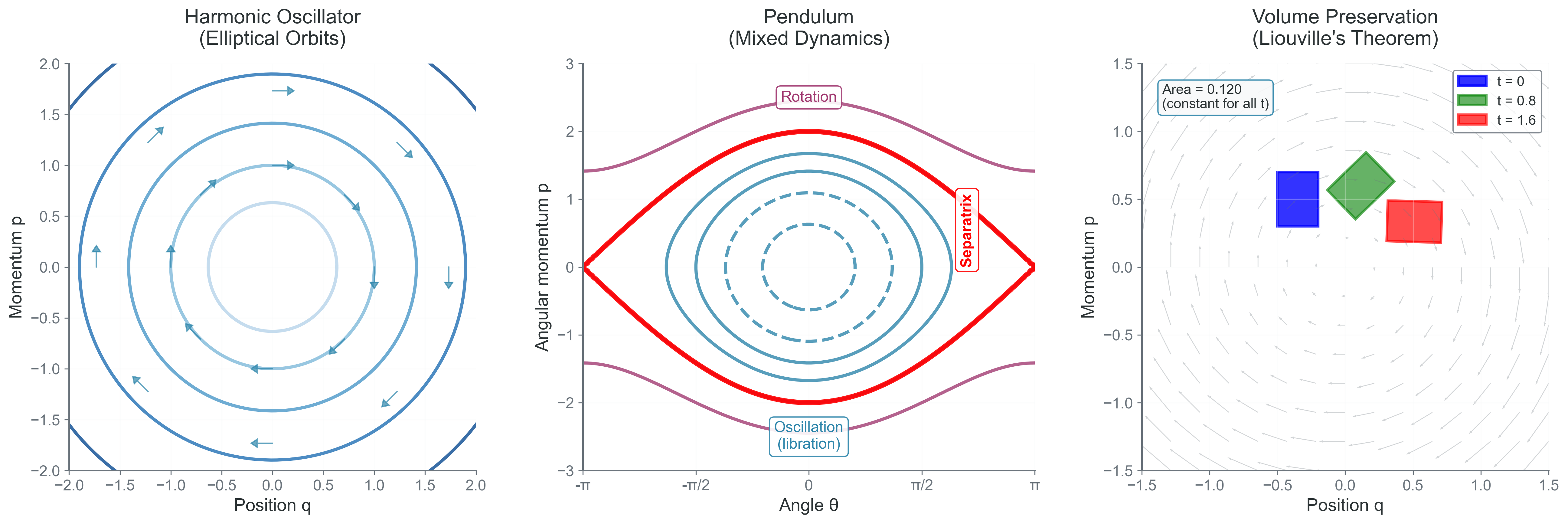
Figure 1:Phase space structure of Hamiltonian systems. (Left) Harmonic oscillator: closed orbits on energy surfaces. (Middle) Pendulum: separatrix divides oscillation from rotation. (Right) Liouville’s theorem: phase space volume is preserved under Hamiltonian flow—areas deform but don’t change size. This geometric structure is what symplectic integrators preserve, ensuring long-term stability.
Liouville’s Theorem
Liouville’s theorem states that phase space volume is preserved under Hamiltonian flow. Mathematically, for a volume element :
This is equivalent to saying the flow is incompressible. Standard numerical methods violate this theorem! They artificially compress or expand phase space, leading to systematic errors.
The Leapfrog/Verlet Method
The leapfrog method (also called Verlet or Störmer-Verlet) staggers position and velocity updates to preserve symplectic structure.
The Algorithm
For a Hamiltonian where :
Why “Leapfrog”?
Positions and momenta “leapfrog” over each other in time:
Time:     t₀    t₁/₂    t₁    t₃/₂    t₂
          |      |      |      |      |
Position: q₀            q₁            q₂
Momentum:       p₁/₂          p₃/₂
This staggering is key to symplecticity!
Implementation Tips for Your N-body Project
Proof of Symplecticity
A transformation is symplectic if it preserves the symplectic 2-form. We’ll prove leapfrog is symplectic by showing each sub-step preserves the symplectic structure.
Step 1: Analyze Each Sub-step
The leapfrog map can be decomposed into three shear transformations:
First kick:
Drift:
Second kick:
Step 2: Show Each Shear is Symplectic
For the momentum kick :
The Jacobian is:
Verify the symplectic condition:
Similarly for the drift step.
Step 3: Composition Preserves Symplecticity
Since the composition of symplectic maps is symplectic:
is symplectic. Therefore, leapfrog preserves phase space structure exactly!
Volume Preservation
The determinant of each Jacobian is 1:
Phase space volume is exactly preserved, satisfying Liouville’s theorem.
The Modified Hamiltonian
Leapfrog doesn’t conserve the original Hamiltonian exactly. Instead, it exactly conserves a modified Hamiltonian:
The correction terms can be computed using backward error analysis. For the harmonic oscillator with :
where is the Poisson bracket.
The key insight: is bounded! Energy oscillates within a band but never drifts away.
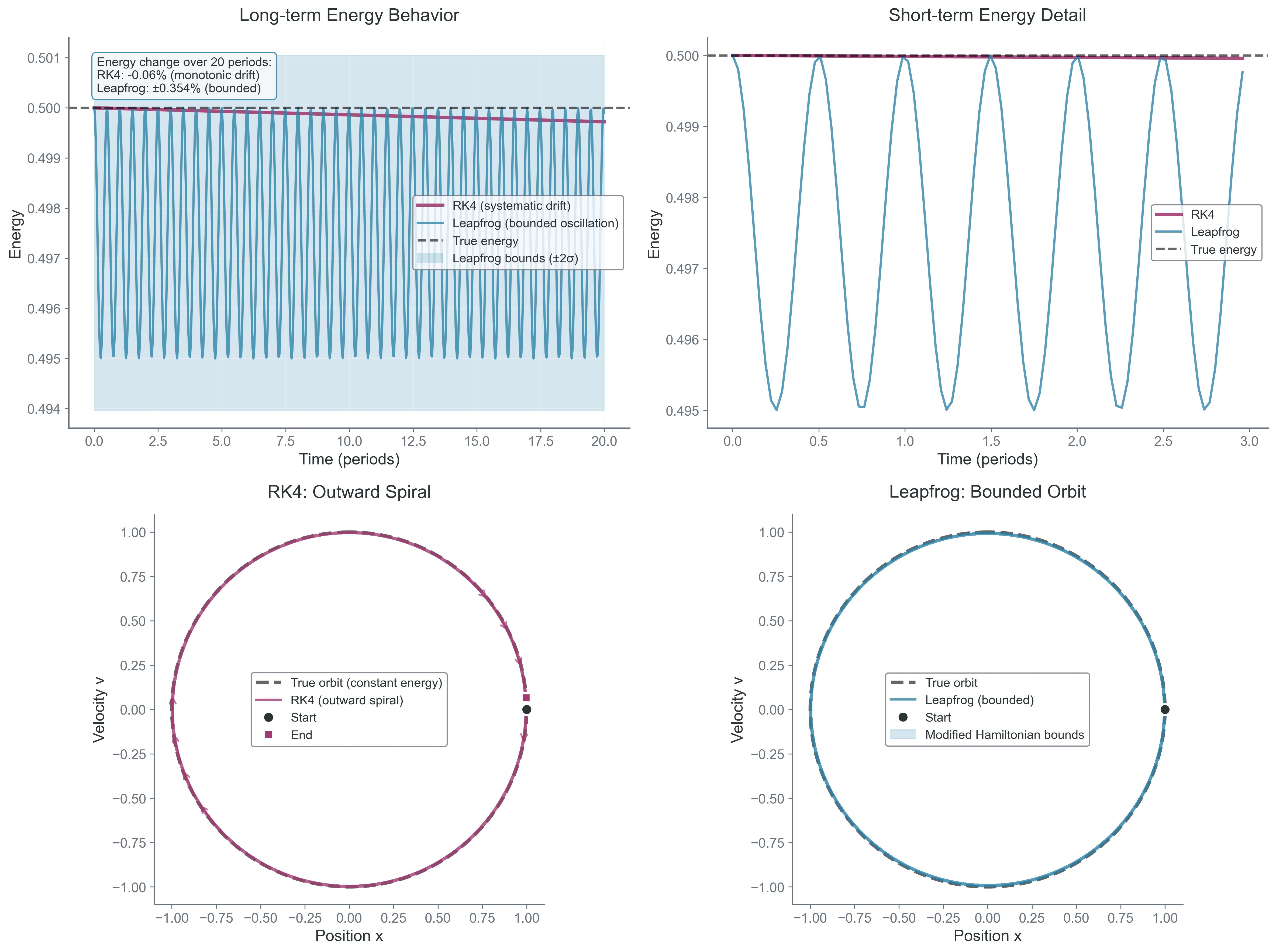
Figure 2:Energy behavior comparison. (Top) RK4 exhibits monotonic energy drift while Leapfrog energy oscillates within bounded envelope. (Bottom) Phase space trajectories: RK4 spirals outward, Leapfrog remains on a nearby invariant torus of the modified Hamiltonian. This demonstrates the fundamental advantage of symplectic methods—trading local accuracy for global stability.
Higher-Order Symplectic Methods
Yoshida’s Fourth-Order Method
By composing leapfrog steps with carefully chosen timesteps, we can achieve higher-order accuracy while maintaining symplecticity. The coefficients come from solving order conditions to eliminate errors.
The strange values involving arise from the algebraic constraints of maintaining symplecticity while achieving fourth-order accuracy:
The algorithm combines leapfrog steps with timesteps where:
Forest-Ruth Method
An alternative fourth-order symplectic integrator with different stability properties. The choice between methods depends on the specific problem’s characteristics.
Performance Comparison: 1000-Year Integration
Testing on Earth’s orbit (eccentricity , period = 365.25 days):
| Method | Order | Energy Error | Phase Error | Stable? |
|---|---|---|---|---|
| Euler | 1 | +100% | 100 radians | No |
| RK2 | 2 | +10% | 10 radians | No |
| RK4 | 4 | +0.1% | 0.1 radians | No |
| Leapfrog | 2 | ±0.01% (bounded) | 0.01 radians | Yes |
| Yoshida4 | 4 | ±0.0001% (bounded) | 0.0001 radians | Yes |
Leapfrog with only second-order accuracy outperforms fourth-order RK4 for long-term stability!
When to Use Symplectic Methods
| Problem Type | Requirement | Best Method | Reason |
|---|---|---|---|
| Solar system (Gyr) | Long-term stability | Symplectic | Bounded energy error |
| Satellite (days) | Trajectory accuracy | RK45 adaptive | Short duration |
| Galaxy merger | Phase space structure | Symplectic | Preserve invariants |
| Molecular dynamics | Energy conservation | Symplectic | 1015 timesteps |
| Dissipative system | Include friction | RK4 | No Hamiltonian structure |
Simple Example: Pendulum Dynamics
Let’s see symplectic integration in action with a nonlinear pendulum:
import numpy as np

def pendulum_leapfrog(theta0, omega0, g, L, h, n_steps):
    """
    Integrate pendulum with leapfrog
    Preserves energy for nonlinear oscillations
    """
    theta, omega = theta0, omega0
    energies = []

    for _ in range(n_steps):
        # Initial energy
        E = 0.5*L**2*omega**2 - g*L*np.cos(theta)
        energies.append(E)

        # Leapfrog update
        omega_half = omega - 0.5*h*(g/L)*np.sin(theta)
        theta_new = theta + h*omega_half
        omega_new = omega_half - 0.5*h*(g/L)*np.sin(theta_new)

        theta, omega = theta_new, omega_new

    return energies
The energy remains bounded even for large amplitude oscillations where linearization fails!
Bridge to Part 4: Stability Analysis
You’ve seen the profound difference between local accuracy and geometric preservation. Symplectic methods sacrifice pointwise precision for global stability, keeping simulations physically meaningful over cosmic timescales.
But choosing the right integrator is only part of the challenge. We also need to understand when methods become unstable, how to diagnose problems, and what limits our timestep choices. In Part 4, we’ll analyze stability regions to predict when methods explode and understand the special challenges of stiff equations.
Next: Part 4 - Stability Analysis