Part 2: Quadrature - From Photon Counts to Dark Matter Halos
Module 2: Static Problems & Quadrature | ASTR 596
Learning Outcomes
By the end of this section, you will be able to:
Derive rectangular, trapezoidal, and Simpson’s rules from Taylor series
Understand optimal point placement through Gaussian quadrature basics
Apply Monte Carlo integration for high-dimensional problems
Choose appropriate methods based on smoothness, dimension, and noise
Analyze error scaling and predict convergence behavior
The Fundamental Challenge
While differentiation is a local operation (needing only nearby points), integration is global—we must consider the entire domain. Quadrature (numerical integration) transforms the continuous integral:
into a discrete sum:
The art lies in choosing:
The points (where to sample)
The weights (how much each sample contributes)
The number (balancing accuracy vs computation)
Physical Motivation: Why Astronomers Integrate
Integration is everywhere in astronomy because we observe integrated quantities:
Spectroscopy: We don’t see individual photons but integrated flux
Photometry: CCD pixels integrate photons over exposure time
Structure: Mass distributions require volume integrals
Cosmology: Distances involve integrating through expanding space
Each context demands different accuracy, and the function properties (smooth vs oscillatory, bounded vs singular) determine the best method.
Building Integration Methods: From Rectangles to Optimality
The Riemann Sum Foundation
The definition of the Riemann integral suggests the simplest approximation:
where and .
Different choices of give different methods:
Left endpoint: Rectangle rule (left)
Right endpoint: Rectangle rule (right)
Midpoint: Midpoint rule
Average of endpoints: Trapezoidal rule
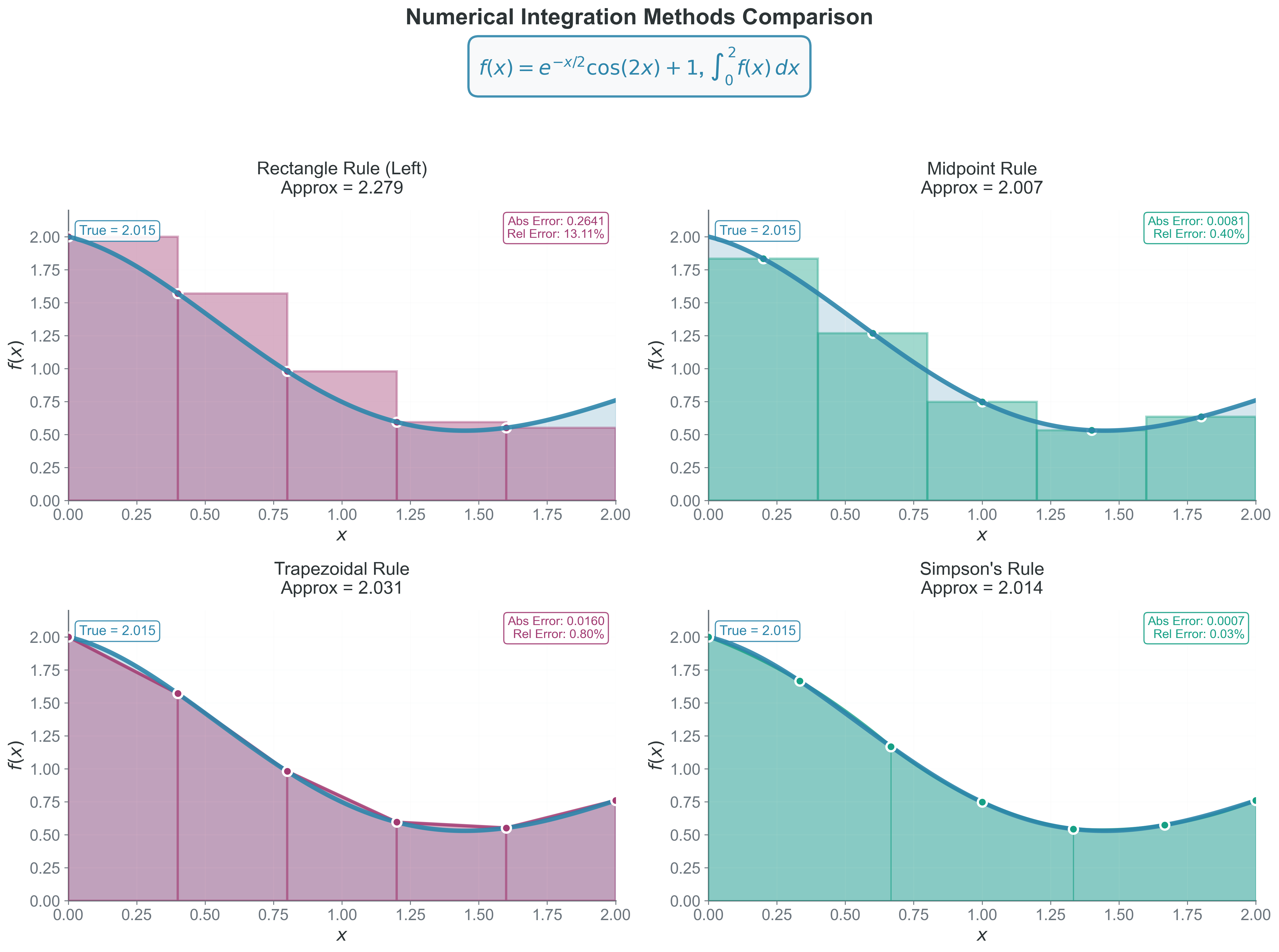
Figure 1:Four geometric approaches to numerical integration. Each method approximates the area under from 0 to 2 using different geometric shapes: Rectangle rule (top-left) uses constant function values at left endpoints, showing systematic error; Midpoint rule (top-right) uses rectangles centered at interval midpoints for better accuracy; Trapezoidal rule (bottom-left) connects function values with straight lines, capturing linear trends; Simpson’s rule (bottom-right) uses parabolic segments through three points, achieving fourth-order accuracy for smooth functions. Each panel displays the true integral value, approximation, and relative/absolute errors. Notice how the colored geometric approximations progressively approach the true area as interpolation becomes more sophisticated—this visual intuition directly corresponds to the mathematical convergence orders.
Method 1: Rectangle Rule - The Starting Point
Why we care: The simplest possible approximation — helps understand error analysis that applies to all methods.
Mathematical Formulation
For uniform spacing :
Error Analysis via Taylor Series
On each subinterval :
Evaluating:
The rectangle rule uses only , so the local error is:
Over intervals:
This is a first-order method—halving halves the error.
Implementation
def rectangle_rule(f, a, b, n):
    """Left rectangle rule"""
    h = (b - a) / n
    total = 0
    for i in range(n):
        x = a + i * h
        total += f(x)
    return h * total
Why Not to Use Rectangle Rule
Only first-order accurate
Systematically over/underestimates for monotonic functions
Poor for oscillatory functions
Mainly pedagogical value
Method 2: Trapezoidal Rule - The Workhorse
Why we care: The workhorse of experimental data integration—robust and simple.
Geometric Intuition
Instead of rectangles, connect consecutive points with straight lines, creating trapezoids. The area of each trapezoid averages the function values at its endpoints.
Mathematical Formulation
The area of a trapezoid with parallel sides and and height is:
Summing over all intervals:
Error Analysis
Using Taylor expansion around the midpoint :
The trapezoidal approximation on :
Since the exact integral is :
Local error:
Global error: for some
This is a second-order method!
Common Failure Modes and Fixes
| Problem | Symptom | Solution |
|---|---|---|
| Singularities | Infinite result | Subtract singularity analytically |
| Oscillations | Poor convergence | Increase n or use adaptive spacing |
| Noisy data | Erratic results | Smooth first or use fewer points |
| Discontinuities | Wrong answer | Split integral at discontinuity |
Method 3: Simpson’s Rule - Parabolic Perfection
Why we care: When your function is smooth and you want high accuracy with moderate computational cost.
The Key Insight
Instead of linear interpolation (trapezoids), use quadratic interpolation (parabolas) through consecutive triplets of points.
Derivation via Interpolation
For three equally-spaced points with and , the unique parabola through is:
Integrating this parabola from to :
These are the famous Simpson weights: 1, 4, 1.
Composite Simpson’s Rule
For intervals (must be even):
The pattern of weights is:
First point: 1
Odd indices (1,3,5,...,n-1): 4
Even indices (2,4,6,...,n-2): 2
Last point: 1
Error Analysis and the Fourth-Order Miracle
Through careful Taylor series analysis, the local error for Simpson’s rule on interval is:
Global error:
Simpson’s rule is fourth-order accurate despite using only parabolas!
Why Simpson’s Rule is Fourth-Order
The “miracle” of Simpson’s fourth-order accuracy comes from symmetry. When we integrate the interpolating parabola, the term (which would give error) has odd symmetry about the midpoint and integrates to zero:
This cancellation is automatic—we get fourth-order accuracy “for free” by using symmetric intervals! Since the error term involves , and the fourth derivative of any cubic polynomial is zero, Simpson’s rule integrates cubic polynomials exactly.
When Simpson’s Rule Shines
Smooth functions with continuous fourth derivative
Periodic functions
When high accuracy is needed with moderate
Functions from physical models (usually smooth)
Common Failure Modes and Fixes
| Problem | Symptom | Solution |
|---|---|---|
| Odd n | Won’t work | Add one interval or use trapezoid for last |
| Noisy data | Amplifies noise | Use trapezoidal instead |
| Discontinuous f⁽⁴⁾ | Poor convergence | Split at discontinuity |
| Sharp peaks | Misses features | Use adaptive refinement |
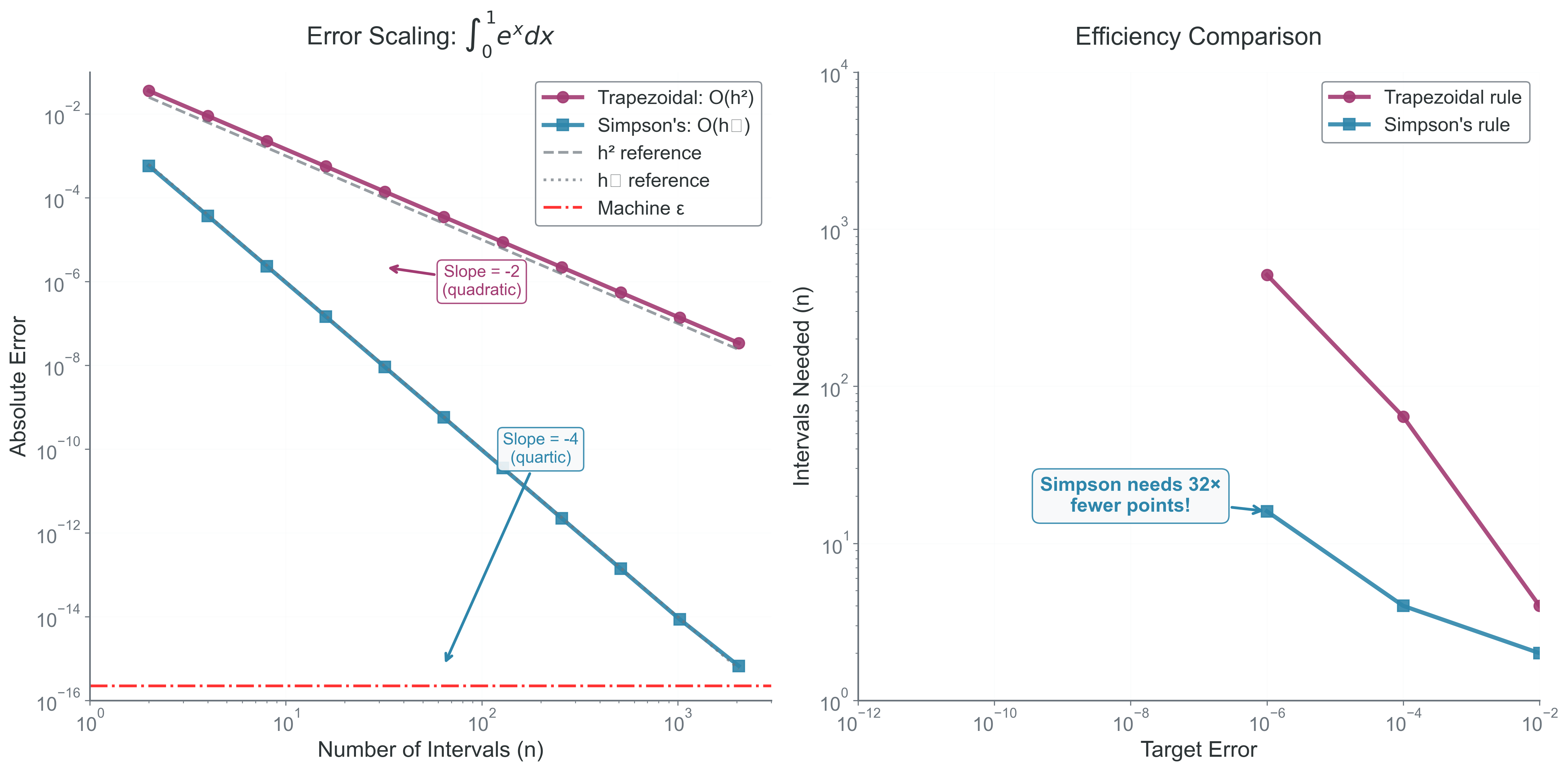
Figure 2:The power of higher-order methods. Comparing error scaling for the integral reveals why Simpson’s rule dominates for smooth functions. Left panel: The log-log plot shows dramatically different convergence slopes—trapezoidal rule’s error decreases as (slope = -2) while Simpson’s rule achieves (slope = -4). Right panel: The efficiency comparison is striking—to achieve 10-10 accuracy, Simpson’s rule needs ~100× fewer points than the trapezoidal rule! This quadratic advantage in computational efficiency explains why high-order methods are preferred for smooth integrands, despite their greater complexity. The machine precision floor () eventually limits both methods, but Simpson’s rule reaches this limit far more efficiently.
Method 4: Gaussian Quadrature - Optimal Point Placement
Why we care: Sometimes being clever about WHERE you sample beats taking MORE samples.
The Revolutionary Idea
All previous methods used equally-spaced points. But what if we could choose both the points AND weights optimally?
Gauss’s insight: For points, we can make the method exact for all polynomials up to degree by choosing specific locations. These points are the roots of Legendre polynomials, which have special orthogonality properties that maximize accuracy.
Example: 2-Point Gaussian Quadrature
Instead of evaluating at equally-spaced points, Gaussian quadrature uses special points. For 2 points on :
Points: ,
Weights:
This seemingly arbitrary choice makes the method exact for all cubic polynomials!
In Practice
You won’t derive Gauss points yourself. Instead:
from scipy.special import roots_legendre

# Get n Gauss points and weights for [-1,1]
points, weights = roots_legendre(n)

# Transform to general interval [a,b]
x_gauss = (b-a)/2 * points + (a+b)/2
w_gauss = (b-a)/2 * weights

# Compute integral
integral = sum(w * f(x) for x, w in zip(x_gauss, w_gauss))
When Gaussian Quadrature Matters
When you control where to sample (not experimental data)
For very smooth functions
When function evaluations are expensive (fewer points needed)
As the foundation for spectral methods in advanced simulations
Key Takeaway: This principle—optimal placement beats more samples—appears throughout computational physics, from choosing timesteps in orbit integration to placing grid points in PDE solvers.
Method 5: Monte Carlo Integration - When Dimensions Explode
Why we care: The only practical method for high-dimensional integrals that appear in statistical mechanics, quantum mechanics, and Bayesian inference.
Understanding Dimensions in Integration
When we talk about “dimensions” in Monte Carlo integration, we mean the number of integration variables, not spatial dimensions:
1D integral: (one integration variable)
2D integral: (two integration variables)
6N-D integral: Phase space integral over N particles with 3 position and 3 momentum components each
For example, computing the partition function for 100 atoms requires a 300-dimensional integral (3 position coordinates per atom)!
The Curse of Dimensionality
For a -dimensional integral with points per dimension, deterministic methods need evaluations:
1D: 100 points
2D: 100² = 10,000 points
3D: 100³ = 1,000,000 points
10D: 100¹⁰ = 10²⁰ points (impossible!)
This exponential growth makes grid-based methods impossible for .
The Monte Carlo Solution
Randomly sample points in the domain :
where is the volume of the domain.
Error Analysis
For the Monte Carlo estimator :
Step 1: The expected value of our estimator is the true integral:
Step 2: The variance of the estimator is:
where is the variance of over the domain.
Step 3: The standard error (standard deviation of the estimator) is:
Key insight: Error independent of dimension !
This assumes:
Independent random samples
Finite variance of the integrand ()
Sufficient samples for CLT to apply (typically N > 30)
When Monte Carlo Wins
| Dimension | Grid Points for 1% Error | Monte Carlo Points for 1% Error |
|---|---|---|
| 1 | 100 | 10,000 |
| 2 | 10,000 | 10,000 |
| 3 | 1,000,000 | 10,000 |
| 5 | 10¹⁰ | 10,000 |
| 10 | 10²⁰ | 10,000 |
Above ~4 dimensions, Monte Carlo becomes superior!
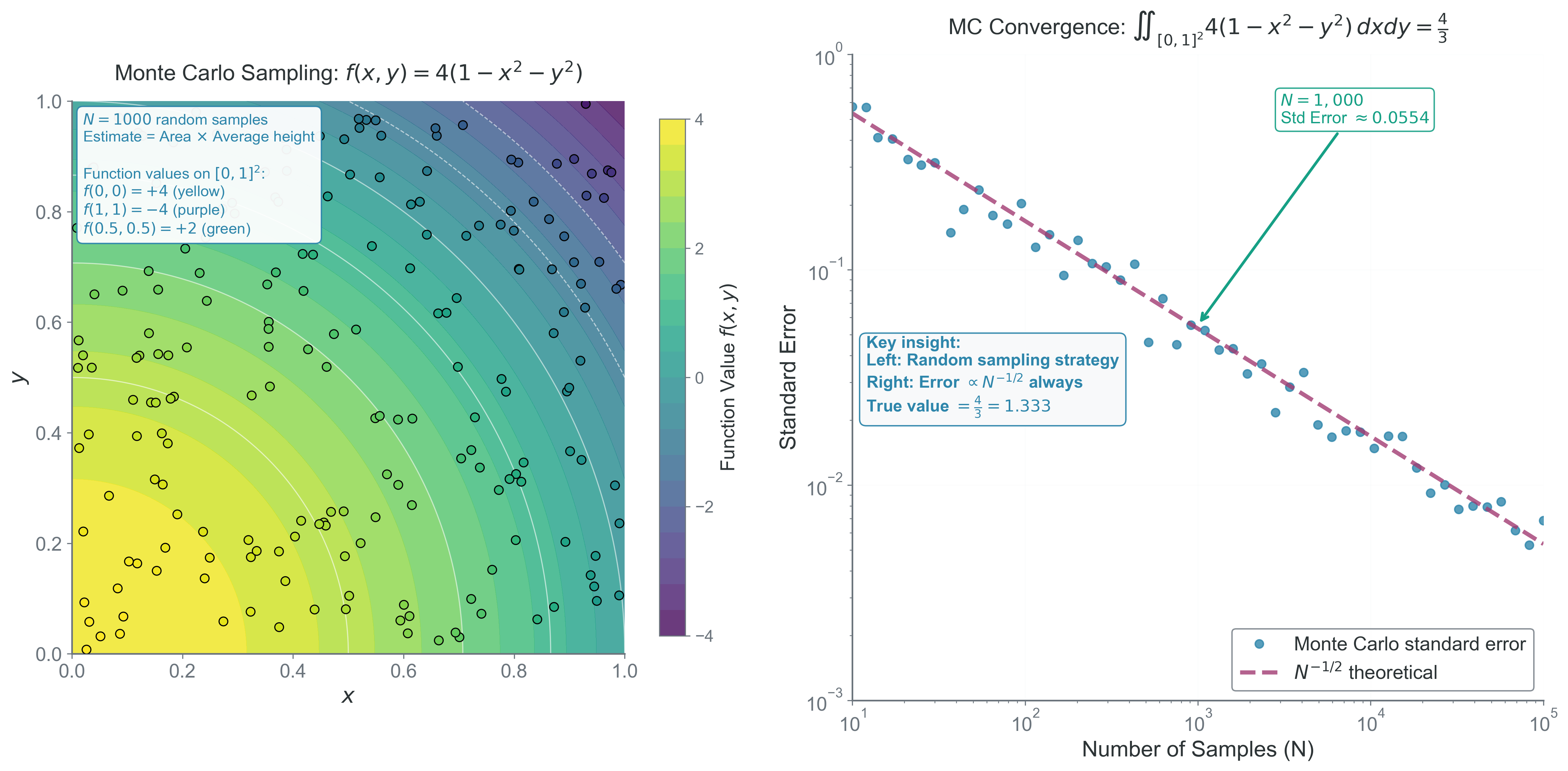
Figure 3:Monte Carlo integration: slow convergence but dimension-independent. Left panel: Unlike grid-based methods, Monte Carlo uses random sampling—here 200 visible points (from 1000 total) sample the 2D paraboloid function over the unit square. Points are colored by function value using the same colormap as the background contours, ranging from (yellow, maximum at origin) to (purple, minimum at corners). The integral estimate equals the domain area times the average function value. Right panel: Statistical convergence analysis from 50 different sample sizes (10 to 100,000), each tested with 20 independent Monte Carlo runs. The standard error (blue points) follows the universal scaling (dashed line) perfectly—this is the fundamental Monte Carlo convergence rate that never depends on dimension , making it revolutionary for high-dimensional integrals in Bayesian inference, quantum mechanics, and statistical mechanics.
Common Failure Modes and Fixes
| Problem | Symptom | Solution |
|---|---|---|
| Infinite variance | No convergence | Use importance sampling |
| Rare events | Poor sampling | Use stratified sampling |
| Correlation | Slower convergence | Use quasi-random sequences |
| Small N | Large uncertainty | Can’t fix—need more samples |
Adaptive Methods and Richardson Extrapolation
Adaptive Quadrature
When functions vary rapidly in some regions but are smooth elsewhere:
def adaptive_simpson(f, a, b, tol):
    """Recursively refine where needed"""
    # Compute with n and 2n points
    I1 = simpson(f, a, b, n=10)
    I2 = simpson(f, a, b, n=20)

    if abs(I2 - I1) < tol:
        return I2
    else:
        mid = (a + b) / 2
        left = adaptive_simpson(f, a, mid, tol/2)
        right = adaptive_simpson(f, mid, b, tol/2)
        return left + right
Richardson Extrapolation
If your method has error , compute at two resolutions:
This cancels the leading error term! For trapezoidal rule (p=2):
This gives fourth-order accuracy from a second-order method!
Real Application: Galaxy Luminosity from Spectrum
Astronomers measure galaxy spectra as discrete samples at wavelengths with fluxes . The total luminosity requires integration:
Challenges
Irregular wavelength spacing from different instruments
Noise in flux measurements
Missing data from atmospheric absorption
Emission lines need high resolution
Solution Strategy
For irregular spacing, use trapezoidal rule with variable h:
def integrate_spectrum(wavelengths, fluxes):
    """Integrate spectrum with irregular spacing"""
    total = 0
    for i in range(len(wavelengths) - 1):
        dλ = wavelengths[i+1] - wavelengths[i]
        f_avg = (fluxes[i+1] + fluxes[i]) / 2
        total += dλ * f_avg
    return total
For emission lines: ensure ~10 points across line width or fit Gaussian profile and integrate analytically.
Choosing the Right Integration Method
Method Comparison Summary
| Method | Order | Pros | Cons | Best For |
|---|---|---|---|---|
| Rectangle | Simple | Inaccurate | Teaching only | |
| Trapezoid | Robust, handles irregular spacing | Moderate accuracy | Experimental data, noisy functions | |
| Simpson | Very accurate for smooth functions | Needs even n, amplifies noise | Smooth theoretical functions | |
| Gaussian | Optimal for polynomials | Need special points | When you control sampling | |
| Monte Carlo | Dimension-independent | Slow convergence | High dimensions (d > 4) |
Practical Guidelines
Start simple: Try trapezoidal first—it often suffices
Check smoothness: Plot your function before choosing
Test convergence: Double n and see if result changes
Consider cost: Is f(x) expensive to evaluate?
Remember libraries: Use
scipy.integrate.quadfor production
Debugging Integration
Common integration bugs and their diagnosis:
| Symptom | Likely Cause | Fix |
|---|---|---|
| Error doesn’t decrease with n | Wrong implementation | Check weights and indices |
| Error plateaus at ~10⁻¹⁴ | Round-off dominance | Use fewer points or extended precision |
| Oscillating convergence | Under-resolving features | Increase n or use adaptive |
| Simpson gives weird results | Odd n | Ensure even intervals |
| Negative result for positive f | Overflow in sum | Use compensated summation |
| Monte Carlo not converging | Infinite variance | Check if σ_f is finite |
Bridge to Part 3: The Unity of Numerical Methods
You’ve now mastered two fundamental classes of problems: finding where functions equal zero and measuring areas under curves. These aren’t isolated techniques—they’re connected by deep mathematical principles.
In Part 3, we’ll explore these connections. You’ll see how root finding and integration are inverse operations, how the same error analysis principles govern both, and how to combine methods for complex problems. Most importantly, you’ll develop the intuition to choose the right method for any computational challenge.
The synthesis ahead will prepare you for the dynamic problems of Module 3, where these static methods become building blocks for simulating evolution through time.
Next: Part 3 - Synthesis