Part 1: The Failure of Naive Integration - ASTR 596: Modeling the Universe

Learning Outcomes¶

By the end of this section, you will be able to:

Implement Euler’s method and witness its catastrophic energy drift
Analyze local vs global error accumulation through Taylor series
Understand why higher accuracy doesn’t guarantee better long-term behavior
Recognize the geometric failure modes in phase space
Predict when and how integration methods will fail

From Continuous to Discrete¶

The fundamental ODE initial value problem asks us to find a function $x(t)$ given its rate of change:

\frac{dx}{dt} = f(x, t), \quad x(t_0) = x_0

(1)

This has the formal integral solution:

x(t) = x_0 + \int_{t_0}^t f(x(s), s) ds

(2)

But this Initial Value Problem contains a circular dependency: to find $x(t)$ , we need to integrate $f(x(s), s)$ , but $f$ depends on the unknown solution $x(s)$ itself!

Numerical methods break this circular dependency by making assumptions about how $f$ behaves over small time intervals:

Constant derivative assumption (Euler): Assume $f$ stays constant over $[t_n, t_{n+1}]$
Linear variation assumption (Trapezoidal): Assume $f$ varies linearly between endpoints
Polynomial approximation (Runge-Kutta): Assume $f$ follows a polynomial of degree $p$

Each assumption leads to a different family of methods with different error behaviors, stability properties, and conservation characteristics.

The Dimensional Analysis of Timesteps¶

Before diving into specific methods, let’s understand what constrains our choice of timestep $h$ from pure dimensional analysis.

For any oscillatory system with characteristic frequency $\omega$ :

Nyquist requirement: $h < π/ω$ (must sample twice per oscillation)
Accuracy requirement: $h < 0.1 × 2π/ω$ (need ~60 points per period)
Typical choice: $h \sim 0.01 × 2π/ω$ (600 points per period)

For gravitational N-body systems, multiple timescales compete:

Orbital period: $t_\text{orb} = 2π\sqrt{(a³/GM)}$ (for semi-major axis a)
Close encounter: $t_\text{coll} = R/(v_\text{rel})$ (where v_rel is relative velocity)
Shortest scale: $t_\text{min} = \min(\text{all pairwise encounter times})$
Required timestep: $h < 0.01 × t_\text{min}$

Example - Earth-Sun system:

Period: $t_\text{orb} = 365.25 \text{ days} = 3.156 × 10⁷ \text{ s}$
Typical timestep: $h \sim 1 \text{ day} = 8.64 × 10⁴$ s
High accuracy: $h \sim 0.1 \text{ day} = 8.64 × 10³$ s

Euler’s Method - The Simplest Approach¶

Mathematical Formulation¶

Euler’s method is the most straightforward discretization possible. Given the ODE

\frac{dx}{dt} = f(x,t),

(3)

at time $t_n$ with solution $x_n$ , and a timestep $h$ , we approximate:

\boxed{x_{n+1} = x_n + h f(x_n, t_n)}

(4)

This assumes the derivative $f$ remains constant over the entire interval $[t_n, t_{n+1}]$ — essentially extending the tangent line at $t_n$ forward by distance $h$ .

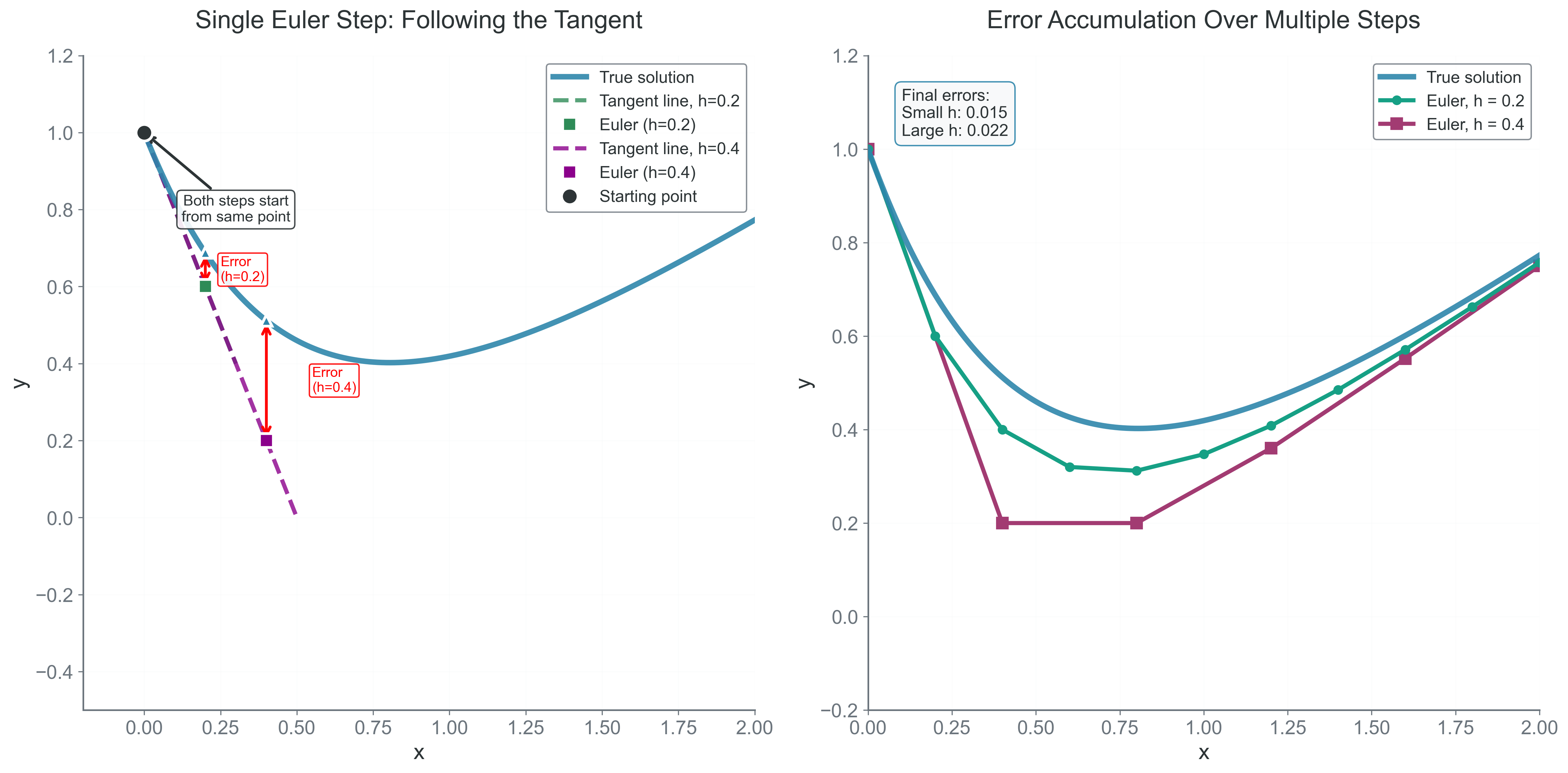
Euler’s method extends the tangent line at each point, accumulating error by ignoring the solution’s curvature. The diagram shows how Euler follows straight line segments (red) that deviate increasingly from the true curved solution (blue). The local truncation error at each step is proportional to h², but these errors accumulate to give O(h) global error. — Figure 1:Euler’s method extends the tangent line at each point, accumulating error by ignoring the solution’s curvature. The diagram shows how Euler follows straight line segments (red) that deviate increasingly from the true curved solution (blue). The local truncation error at each step is proportional to $h²$ , but these errors accumulate to give $O(h)$ global error.

Taylor Series Analysis of Error¶

To understand Euler’s error precisely, we need the Taylor series. The true solution at $t_{n+1} = t_n + h$ is:

x(t_n + h) = x(t_n) + h x'(t_n) + \frac{h^2}{2}x''(t_n) + \frac{h^3}{6}x'''(t_n) + O(h^4)

(5)

Since $x'(t_n) = f(x(t_n), t_n)$ by definition of our ODE, Euler’s method gives:

\boxed{x_{n+1} = x_n + h f(x_n, t_n)}

(6)

The local truncation error — the error in one step — is:

\tau_n = x(t_{n+1}) - x_{n+1} = \frac{h^2}{2}x''(t_n) + O(h^3)

(7)

The leading error term is $O(h^2)$ , making Euler locally second-order accurate. But errors accumulate! Over $N = t_\text{final}/h$ steps to reach final time $t_\text{final}$ , the global error becomes:

E_\text{global} = \sum_{i=0}^{N-1} \tau_i \approx N \cdot \frac{h^2}{2}x''(\xi) = \frac{t_\text{final}}{h} \cdot \frac{h^2}{2}x''(\xi) = \frac{t_\text{final} h}{2}x''(\xi) = O(h)

(8)

Euler is globally first-order: halving the timestep only halves the total error.

The Energy Drift Catastrophe¶

Let’s see Euler fail catastrophically on the harmonic oscillator:

\ddot{x} = -\omega^2 x

(9)

Converting to first-order system:

\frac{d}{dt}\begin{pmatrix} x \\ v \end{pmatrix} = \begin{pmatrix} v \\ -\omega^2 x \end{pmatrix}

(10)

The true solution has constant energy $E = \frac{1}{2}(v^2 + \omega^2 x^2).$

Implementation and Analysis¶

import numpy as np

def euler_harmonic(x0, v0, omega, h, n_steps):
    """Integrate harmonic oscillator with Euler's method"""
    x, v = x0, v0
    E0 = 0.5 * (v0**2 + omega**2 * x0**2)
    
    energies = [E0]
    for i in range(n_steps):
        # Euler update
        a = -omega**2 * x
        x = x + h * v
        v = v + h * a
        
        # Energy (should be constant, but...)
        E = 0.5 * (v**2 + omega**2 * x**2)
        energies.append(E)
    
    return energies

The shocking result: energy grows approximately linearly with time! After 1000 orbital periods, energy has typically increased by 10%. The orbit spirals outward, violating conservation of energy.

Mathematical Analysis of Energy Growth¶

For the harmonic oscillator with Euler’s method, we can derive the exact energy growth rate. Starting with position $x_n$ and velocity $v_n$ :

x_{n+1} = x_n + hv_n

(11)

v_{n+1} = v_n - h\omega^2x_n

(12)

The energy after one step:

E_{n+1} = \frac{1}{2}(v_{n+1}^2 + \omega^2 x_{n+1}^2)

(13)

Substituting the updates:

E_{n+1} = \frac{1}{2}[(v_n - h\omega^2x_n)^2 + \omega^2(x_n + hv_n)^2]

(14)

Expanding:

E_{n+1} = \frac{1}{2}[v_n^2 - 2h\omega^2x_nv_n + h^2\omega^4x_n^2 + \omega^2x_n^2 + 2h\omega^2x_nv_n + h^2\omega^2v_n^2]

(15)

E_{n+1} = \frac{1}{2}[v_n^2 + \omega^2x_n^2] + \frac{h^2\omega^2}{2}[v_n^2 + \omega^2x_n^2]

(16)

Therefore:

\boxed{E_{n+1} = E_n(1 + h^2\omega^2)}

(17)

The amplification factor $(1 + h^2\omega^2) > 1$ means energy grows exponentially! After $N$ steps:

E_N \approx E_0(1 + h^2\omega^2)^N \approx E_0 e^{Nh^2\omega^2} = E_0 e^{t_\text{final}h\omega^2}

(18)

For Earth’s orbit with $h = 1$ day and $t_\text{final} = 1000$ years:

\frac{E_{final}}{E_0} \approx e^{0.1} \approx 1.1

(19)

A 10% energy increase means that Earth would drift into a higher orbit!

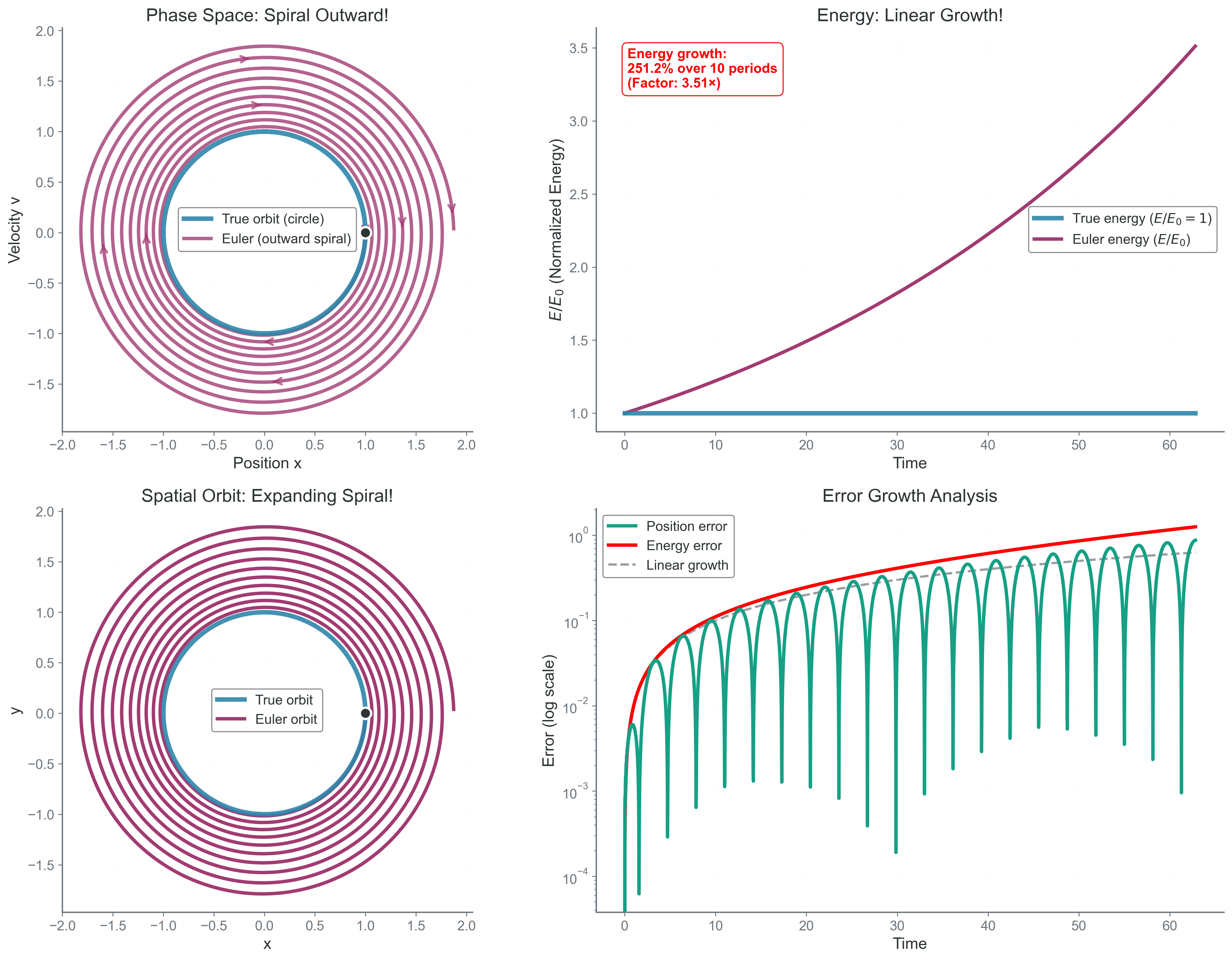
Figure 2:Euler’s method systematically violates energy conservation with catastrophic consequences. The figure shows a harmonic oscillator integrated over 10 periods with timestep h = 0.02: (Top left) Phase space trajectory spirals outward as energy increases ~3.5×. (Top right) Energy grows monotonically from amplification factor (1 + h²ω²) ≈ 1.0004 per step compounding over many orbits. (Bottom left) Spatial orbit expands continuously—a planet would spiral away from its star! (Bottom right) Error analysis shows systematic energy injection (red line) versus oscillating position errors (teal). This demonstrates why Euler fails for long-term dynamics despite being locally accurate.

Why Euler Fails: The Geometric View¶

In phase space (position-velocity space), the harmonic oscillator traces a circle. Each Euler step moves along the tangent to the circle, placing the new point slightly outside. The phase space area increases, violating Liouville’s theorem that phase space volume must be preserved in Hamiltonian systems.

The Phase Error Problem¶

Even if we could tolerate energy drift, Euler has another fatal flaw: phase error. The frequency of oscillation is wrong:

\omega_{numerical} = \omega_{true}(1 + O(h^2))

(20)

After $N = t_\text{final}/h$ oscillations, the phase error is:

\Delta\phi = N \cdot O(h^2) = \frac{T}{h} \cdot O(h^2) = O(h)

(21)

This means that even with small timesteps, the phase error accumulates linearly with time.

When Does Euler Work?¶

Despite these failures, Euler has legitimate uses:

Very short integrations where $N h^2 \ll 1$
Highly dissipative systems where energy should decay
Quick explorations before using better methods
Teaching why better methods are needed!

The Fundamental Lesson¶

Euler’s method reveals a profound truth about numerical integration:

Local accuracy does not guarantee global stability

Euler is locally second-order accurate ( $O(h^2)$ per step), yet it systematically violates conservation laws. This isn’t a bug — it’s a fundamental property of the discretization.

The tangent line approximation, while locally accurate, doesn’t respect the curved geometry of phase space. Each step compounds this geometric error until the qualitative behavior is wrong.

Bridge to Part 2: The Quest for Better Methods¶

Euler’s catastrophic failure motivates our search for better integration methods. The failure isn’t just about accuracy — it’s about systematic bias. Every Euler step pushes slightly outward from the true trajectory. This accumulation of geometric errors destroys the physics we’re trying to simulate.

What we need are methods that:

Sample the derivative at multiple points to cancel biases
Achieve higher-order accuracy to reduce error accumulation
Maintain stability over long integration times
Preserve conservation laws or at least bound their violation

In Part 2, we’ll explore the Runge-Kutta family — methods that evaluate the derivative at carefully chosen intermediate points to achieve higher accuracy. By sampling the “curvature” of the solution, these methods can follow the true trajectory more faithfully. But as we’ll discover, even fourth-order accuracy isn’t enough to preserve energy over cosmic timescales.

The journey from Euler to modern integration methods is a journey from naive approximation to deep understanding of geometric structure. Each method we develop addresses specific failures of its predecessors, leading ultimately to symplectic integrators that preserve the fundamental geometry of physics.

Next: Part 2 - Building Better Methods