When should we trust a numerical answer?¶
Last time: build a root finder and explain its stopping rule.
Today: propose → test → accept or revise → verify.
We will connect each advanced method to the problem it helps solve.
Recall · what does “small” mean?¶
Residual magnitude: ∣f(xn)∣ measures equation mismatch; a signed residual keeps the sign.
Update: sn=∣xn−xn−1∣ measures the last move.
Bracket: a valid [an,bn] containing x∗ bounds midpoint error:
Pair prompt: which assumptions turn each observation into evidence?
Why go beyond the basic methods?¶
The basic methods show how approximation, iteration, and stopping work.
Advanced methods become useful when:
A fast local step is unreliable from your starting guess.
Each function evaluation is expensive.
You fit many observations with a few parameters.
An integrand has structure that uniform sampling resolves inefficiently.
Goal: recognize the problem, choose a method, and check its answer.
Ask what information the problem gives you¶
| What you have | What it enables |
|---|---|
| A continuous function and opposite endpoint signs | Bracket-based root control |
| Slopes or a local linear approximation | Fast trial steps |
| Predictions and observations | A least-squares objective |
| A callable integrand | Choosing new sample locations |
Discuss: if you only have fixed sampled data, can you freely choose Gaussian nodes?
A local model of f(x) proposes a step¶
The tangent line near xn is our local model of f(x):
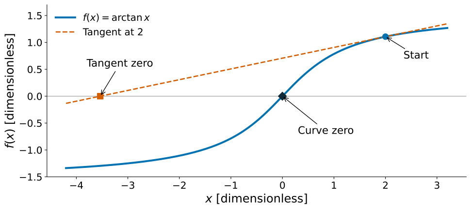
Predict: Newton proposes the line’s zero. Will this step reduce ∣f(x)∣?
Separate direction from distance¶
Direction: Newton supplies p.
Step length: a line search chooses α.
Trial rule: try the full step; shorten it if the acceptance test fails.
Define progress before accepting a step¶
Use a residual objective: ϕ(x)=21f(x)2.
For an exact Newton direction at a nonroot,
A short enough step decreases this objective under the differentiability assumptions. A full step may not.
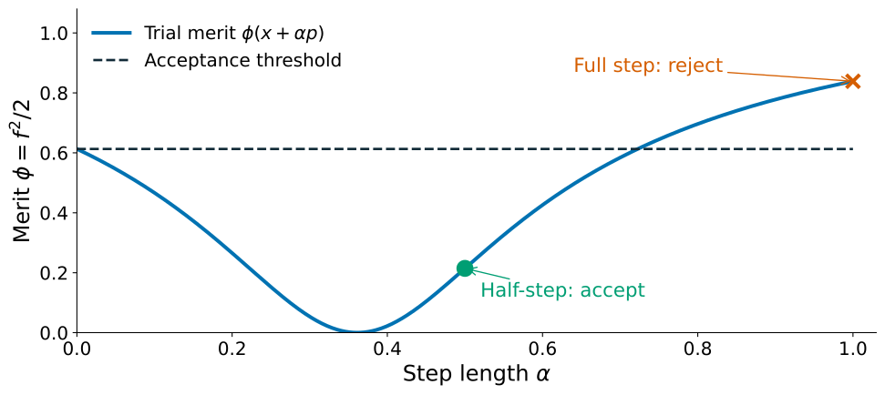
Demonstration · compare the trial steps¶
For f(x)=arctanx at x=2, the initial residual magnitude is 1.107.
| Step fraction α | Trial input | Residual magnitude | Sufficient decrease? |
|---|---|---|---|
| 1 | -3.536 | 1.295 | No |
| 1/2 | -0.768 | 0.655 | Yes |
| 1/4 | 0.616 | 0.552 | Yes |
Backtracking accepts the first passing trial. It need not find the best step.
Explain: why is acceptance not convergence?
When is a line search useful?¶
Use when: a local direction is promising but the full step overshoots.
Example: nonlinear calibration from an uncertain starting guess.
Check: actual objective decrease, not just the tangent’s prediction.
Cost: rejected trials require extra evaluations.
Limit: shorter steps cannot create a root. Check the domain, residual, and stopping conditions.
A bracket gives a different kind of protection¶
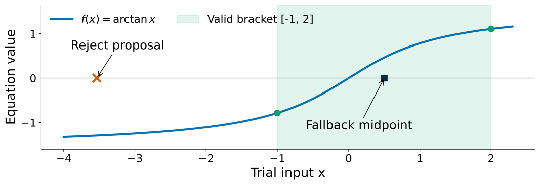
Predict: which endpoint should be replaced after evaluating f(0.5)>0?
Keep opposite signs. A fallback bisection step reduces the bracket width.
Safeguarded methods · fast proposals, controlled progress¶
Use a hybrid method when you have a valid bracket and want faster progress than bisection alone.
Propose a fast step using local information.
Check that it is safe and makes adequate progress.
Otherwise, take a bracket-reducing step.
Brent-type methods combine interpolation and bisection; the preceding tangent example illustrates the safeguard idea, not Brent’s exact algorithm.
Continuity and reliable signs still matter.
From roots to fitting data¶
A residual is prediction minus observation: ri(θ)=g(ti;θ)−yi.
Choose parameters θ to reduce Φ(θ)=21∑iri(θ)2.
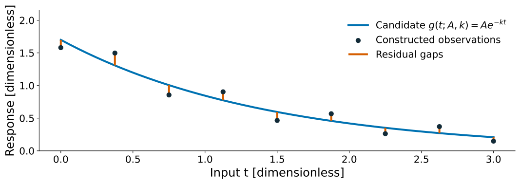
Noisy observations generally cannot all have zero residual.
The Jacobian · one slope for each input–output pair¶
Let r(θ) have m outputs and θ have n parameters.
Row: one output’s sensitivity to all parameters.
Column: all outputs’ sensitivity to one parameter.
A partial derivative changes one parameter while holding the others fixed.
The matrix is a local input–output map¶
For a small parameter update p,
The dimensions tell us what this means:
Component by component: Δri≈∑jJijpj.
Each entry has units “output i per unit of parameter j.”
Predict: is the Jacobian necessarily square?
Example · three observations, two parameters¶
Fit g(t;A,k)=Ae−kt to fixed observations yi at t=0,1,2.
For ri=Ae−kti−yi,
Evaluate the slopes at the current parameters¶
Rows: observation times t=0,1,2.
Columns: parameters A and k.
Explain: why is the top-right entry zero?
Use the Jacobian to predict a change¶
Increase A by 0.10 and k by 0.02:
These are predicted changes in residuals, not the residuals themselves.
Increasing amplitude raises the curve; increasing decay rate lowers later values. The effects partly cancel.
Check: compare r(θ+p)−r(θ) with Jp, then reduce the step.
Check the local prediction against the actual change¶
For p=(0.10,0.02), evaluate the exponential again:
| Time | Predicted Jp | Actual change |
|---|---|---|
| 0 | 0.100000 | 0.100000 |
| 1 | 0.030000 | 0.029209 |
| 2 | 0.005000 | 0.004414 |
For 0.1p, the largest discrepancy falls from 7.91×10⁻⁴ to 7.99×10⁻⁶: about 99× smaller.
Explain: why does shrinking the step improve this linear prediction?
Read the least-squares notation¶
Transpose exchanges rows and columns:
Squared norm adds squared entries:
Gradient: ∇θΦ has one loss derivative per parameter.
Nonsingular: a square matrix for which every right-hand side has exactly one solution.
J describes separate outputs; ∇Φ describes one scalar loss.
DS/ML · from many outputs to one loss¶
For least-squares loss Φ(θ)=21r(θ)Tr(θ),
The Jacobian describes how parameters affect predictions; the loss gradient combines those effects into one direction of change.
Where it appears: nonlinear regression, calibration, and sensitivity of model predictions.
Backpropagation applies the chain rule through a model. It can compute products such as JTr without storing the full Jacobian.
This connection does not mean neural networks are usually trained with Levenberg–Marquardt.
Computational science · coupled equations¶
A steady state or implicit time step can require solving F(u)=0 for many unknowns.
Linearize the coupled equations:
For a square, nonsingular Jacobian, Newton’s proposal solves
Examples: chemical equilibrium and coupled transport equations. Inverse problems instead often fit observations by minimizing a loss.
The Jacobian shows which variables affect which equations. Weak or dependent sensitivities can make the solve difficult.
Gauss–Newton · fit the local residual model¶
For a root, Newton sets a local approximation to zero.
For a fit, Gauss–Newton minimizes its squared mismatch:
At a minimizer, JTJp=−JTr.
A local fit can propose a large step where the approximation is poor.
Next question: can we discourage such large steps?
Derive a penalty on the proposed step¶
1. Define the penalized local fit in scaled parameters:
2. Differentiate with respect to the update p:
3. Solve where the gradient is zero:
The penalty limits the current step; it does not require parameters near zero.
Levenberg–Marquardt · damp the local fit¶
Local model: r(θ+p)≈r(θ)+Jp.
Levenberg step:
Jacobian: Jij=∂ri/∂θj.
Update: p changes the parameters.
Damping: λ>0 controls the penalty.
Identity: I leaves a vector unchanged.
Marquardt variants add scaling.
Accept only after checking: evaluate the actual fit improvement.
Read the contour plot before comparing steps¶
Contours: equal local squared mismatch.
Cross: the local-model minimum.
Arrows: alternative damping choices from the same starting point, not successive iterations.
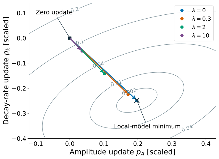
Damping changes the proposed direction¶
Small damping: near the Gauss–Newton step when JTJ is nonsingular.
Large damping: p≈−JTr/λ, a small gradient-like step.
Predict: does a tiny update establish a good fit?
When is Levenberg–Marquardt useful?¶
Use when: fitting smooth nonlinear models by least squares.
Example: calibration, decay curves, or parameter fitting.
Check: actual loss reduction, residual patterns, and parameter sensitivity.
Limit: a small residual does not establish unique or well-determined parameters.
Trial rule: scale parameters sensibly; adjust damping after checking each trial.
Decision case · fitting a decay curve¶
You fit noisy observations with Ae−kt from a poor initial guess.
Poor local prediction: damp the trial; compare predicted and actual loss reduction.
Different parameter scales: choose meaningful scales before applying λI.
Only very early observations: sensitivity to k is weak because ∂g/∂k=−Ate−kt.
Discuss: can damping replace later observations that constrain the decay rate?
A stable numerical step does not establish that the data identify both parameters.
Three different ways to control a step¶
Line search: shorten a direction until it produces sufficient decrease.
Bracket safeguard: retain a valid bracket and replace unsafe proposals.
Levenberg damping: change the linear system proposing the direction.
Invariant: only the bracketed method carries a root bracket.
Integration · check the error model too¶
Adaptive quadrature: refine where local estimates indicate difficulty.
Richardson: cancel a leading error term when its expansion applies.
Predict: can two estimates agree because both missed the same feature?
Smaller reported error is evidence to investigate, not an unconditional certificate.
Where should we spend the next evaluation?¶
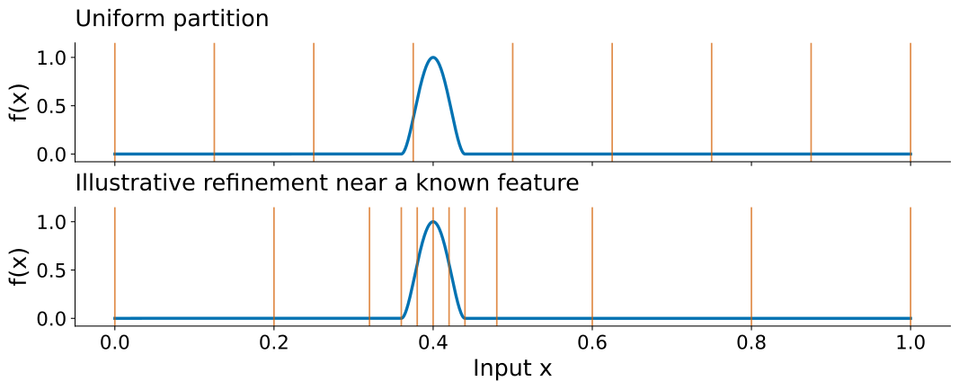
Uniform refinement: sample everywhere.
Local refinement: concentrate samples where needed.
The partition uses a known feature location; it is not an adaptive solver trace.
Agreement can mean that both estimates missed it¶
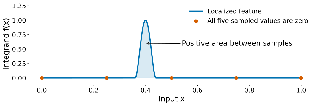
Predict: what would coarse and refined rules report if both only see zeros?
Use known feature locations, interval splitting, and independent checks. An error estimator only sees what was sampled.
Richardson · use the error pattern¶
1. Assume Q(h)=I+Chp+higher-order terms.
2. Refine to Q(h/2)=I+Chp/2p+⋯.
3. Cancel the leading error:
Symbols: h is spacing; p is leading error order; I is the integral.
Predict: why would the wrong p spoil cancellation?
Richardson works when the assumed pattern applies¶
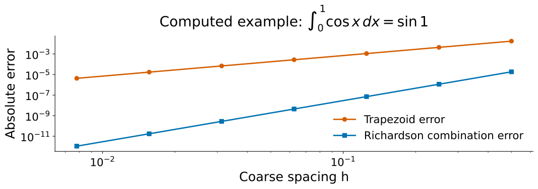
Useful when a smooth problem has a stable error expansion at these resolutions.
Sharp features, insufficient resolution, or rounding can break that pattern.
Gauss–Legendre · choose nodes and weights¶
Nodes: xi specify where to evaluate. Weights: wi set each contribution.
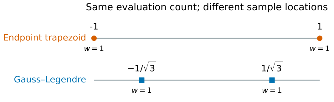
Predict: for f(x)=x2, which sample locations give a better integral?
Two evaluations · compare the answers¶
For f(x)=x2, the exact integral on [−1,1] is 2/3.
Endpoint trapezoid: QT=f(−1)+f(1)=2.
Two-node Gauss–Legendre:
With n nodes, Gauss–Legendre is exact for polynomials through degree 2n−1 in exact arithmetic.
Limit: two nodes handle cubics exactly, but not every function. What check would you use for a new integrand?
See what the two rules measure¶
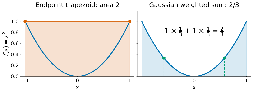
Left shading: trapezoid approximation.
Right shading: true integral.
Gaussian weights combine sampled values; they are not automatically widths of little panels.
When is Gauss–Legendre useful?¶
Use when: a smooth function can be evaluated at chosen nodes.
Example: an expensive integrand on a finite interval.
Check: compare orders or split the interval.
Limit: no built-in error estimate; treat discontinuities and endpoint singularities explicitly.
Exactness: n nodes integrate polynomials through degree 2n−1 in exact arithmetic. This does not extend to every smooth function.
Fixed measured samples usually require a different approach.
Map the nodes to your interval¶
Library nodes xi and weights wi are defined on [−1,1].
1. Map nodes to [a,b]:
2. Scale weights by half the interval length:
Check: for f=1, the answer must be b−a. Both transformations matter.
Convergence · which quantity contracts?¶
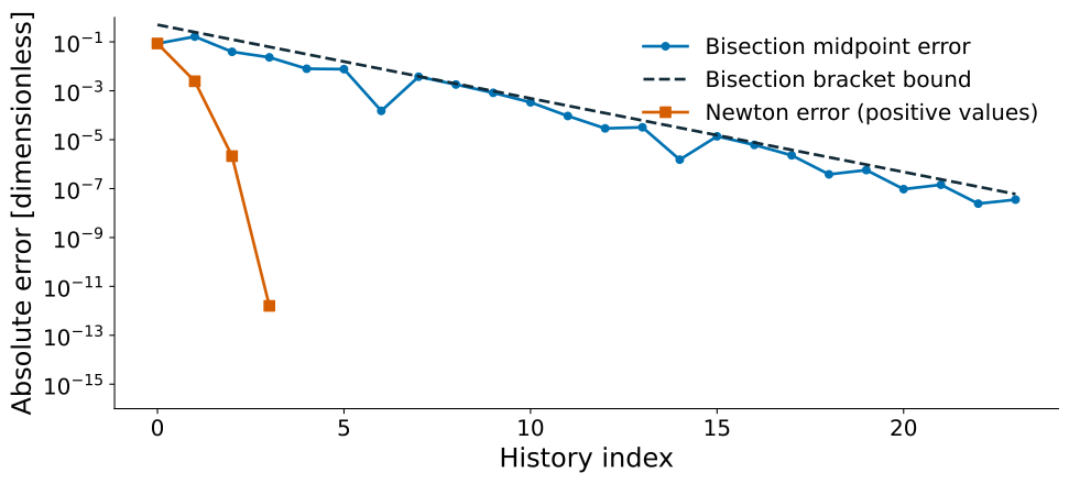
Predict: can a midpoint become worse while its bracket becomes better?
Estimate order from three errors¶
Suppose consecutive errors are 10−1,10−2,10−4.
Three errors support this estimate. A zero error cannot enter the logarithm.
A short triple suggests local behavior; it does not prove asymptotic order.
A bracket measures something different¶
Widths 1,1/2,1/4,1/8 have ratio 1/2.
The slope of log width against iteration is −log2.
Actual midpoint errors need not decrease at every update.
Pair task: return to the convergence plot. Identify three consecutive positive Newton errors suitable for an order estimate. Find a bisection update where midpoint error rises while its bracket bound halves.
Fast convergence is not the same as low cost¶
Compare work at the same meaningful accuracy.
Count:
Function evaluations, including rejected trials.
Derivative evaluations.
Linear-system solves.
A higher-order quadrature rule uses more nodes per call. Cost also depends on what each evaluation computes.
Discuss: when could fewer iterations take longer?
Choose a method and a check¶
For one case, propose a method and an independent check:
A continuous scalar equation with a sign-changing bracket.
A nonlinear curve fitted to noisy observations.
An integral with a known narrow feature.
Project 3 will implement and apply bisection, Newton, and secant. Today’s advanced methods are an overview.
Project 2 · protected work time¶
Due Wednesday, September 23, 11:59 pm PT
Choose your first unresolved check:
Separate cutoff error from quadrature refinement.
Recover the uniform-disk limit.
Explain convergence near a branch point.
Compare adaptive accuracy with actual evaluation counts.
Show the predicted result, measured result, and the smallest case that disagrees.
the acceptance rule¶
Armijo sufficient decrease:
The example uses c=10−4 and halves α after rejection.
These are step-control settings, not root-accuracy tolerances. The reading contains the derivation and failure contract.
what a line search cannot promise¶
The merit function can have a stationary point with f=0.
For f(x)=x2+1, no real root exists, although ϕ has a minimum at zero.
Inspect the equation, domain, and sensitivity. Treat stagnation and exhausted budgets as failures, not successful convergence.
Method overview¶
FNC §4.6 · Quasi-Newton methods: focus on Levenberg’s method and the damped system.
FNC §5.7 · Adaptive integration: error estimation and adaptive refinement.
FNC §9.6 · Spectrally accurate integration: focus on Gauss–Legendre integration and the two-node example.
Optional conceptual follow-up; textbook implementations do not replace your project code.
SciPy’s least-squares documentation describes method="lm" (Levenberg–Marquardt). It does not support parameter bounds.
Course readings: Backtracking, Hybrid Methods, Adaptive Methods and Richardson Extrapolation.
Gaussian nodes in Python¶
NumPy leggauss(n) returns n nodes and weights on [−1,1].
SciPy roots_legendre(n) provides the same ingredients, with a worked interval-mapping example.
These functions do not evaluate your integrand or return its integral. You evaluate the function and form the weighted sum.
Optional exploration; does not replace required project implementations.
PyTorch: Jacobians and Jacobian products explains the automatic-differentiation connection.