From geometric steps to reusable code
Approximate a slope using function values and Taylor expansion.
Rebuild Newton’s update, then reuse information in secant.
Interpret small quantities before declaring convergence.
Build a module whose tests check the mathematical contract.
Jump to: Finite differences · Newton to secant · Stopping · Module activity · Advanced reference
Today’s question
How do we turn a root-finding formula into a result we can explain?
Recall quantile inversion: solve C(x)−q=0. Each new target probability q requires another solve.
Equilibrium models and implicit ML predictions also reuse root finders. We need accuracy evidence and clear failure behavior.
Today: approximate a slope → reuse values → decide when to stop → build a tested module.
Recall bisection: keep a root bracketed
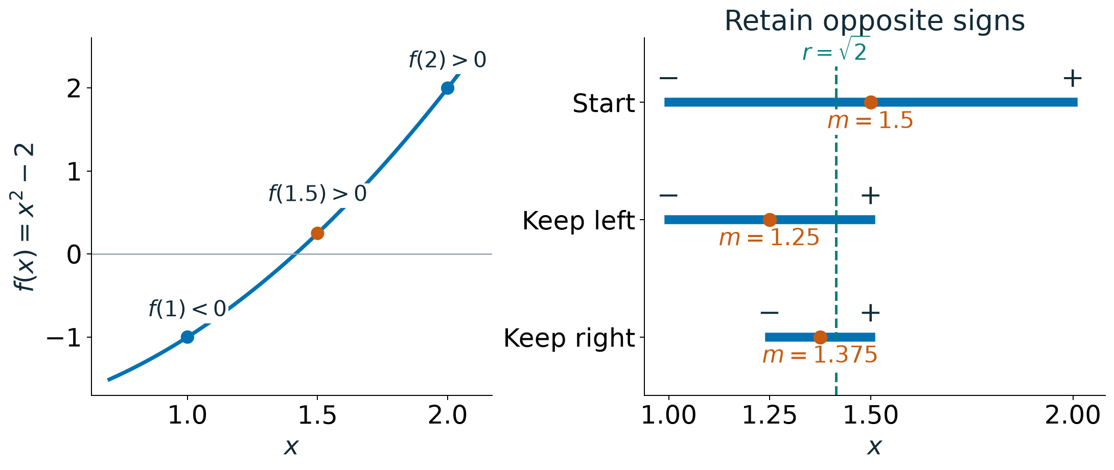
For continuous f, retain opposite endpoint signs to keep a root r bracketed. Evaluate m; retain a half; repeat.
Can local shape suggest the next input?
Bisection uses signs to retain a bracket. Newton uses a local slope to propose a new input.
To use a slope, we first need to understand how a computer approximates a derivative from function values.
Route: approximate a derivative → rebuild Newton’s update → reuse samples in secant.
I · Approximate a derivative from values
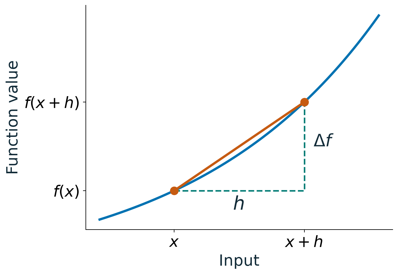
What if we can evaluate f, but have no derivative routine?
Use two nearby values:
As h→0, this secant slope tends to f′(x) when the derivative exists.
A computer uses h=0. Taylor expansion explains the error.
Taylor explains the derivative error
For sufficiently smooth f near x,
Subtract f(x) and divide every remaining term by h=0:
When f′′(x)=0, the leading error is first order: halving h approximately halves it. Derivation reference.
Predict: is the smallest step best?
For f(x)=ex at zero, the exact derivative is 1.
# lecture-example: difference
import numpy as np
steps = 10.0 ** (-np.arange(1, 17))
slopes = (np.exp(steps) - 1.0) / steps
errors = np.abs(slopes - 1.0)
for h, slope, error in zip(steps[::3], slopes[::3], errors[::3]):
    print(f"h={h:.0e}: slope={slope:.8f}, error={error:.2e}")
arange excludes 17. np.abs measures error; zip pairs entries. [::3] prints every third step.
Predict: which step gives the smallest error? Run, then compare with the next plot.
Smaller helps until rounding interferes
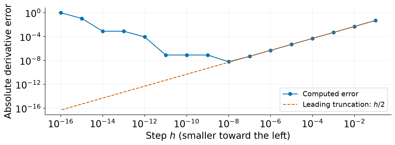
Read leftward for smaller steps. Rounding eventually outweighs the reduction in truncation error.
Two errors pull the step size in opposite directions
Truncation
Write Dhf=[f(x+h)−f(x)]/h. Forward difference drops Taylor terms:
Smaller h reduces this error in the smooth regime.
Floating-point effects
The function values are rounded. Subtracting nearby values exposes those errors; division by h magnifies them.
A common model is
Here ε denotes machine precision. The constants depend on the function and its scale; there is no universally best fixed step.
II · From Newton to secant
Near the current estimate xk, replace the curve by its tangent model:
Set ℓk(xk+1)=0 and solve for the correction:
Here k counts updates, f(xk) is the residual, and f′(xk) is the local slope. We solve the linear model exactly; the curve is only approximated.
Predict Newton’s next input
For f(x)=x2−2, use f′(x)=2x and start at x0=2.
Predict: where does the tangent cross zero? Is the original curve also zero at that input?
What must we recompute before taking another step?
Watch Newton calculate, move, and rebuild
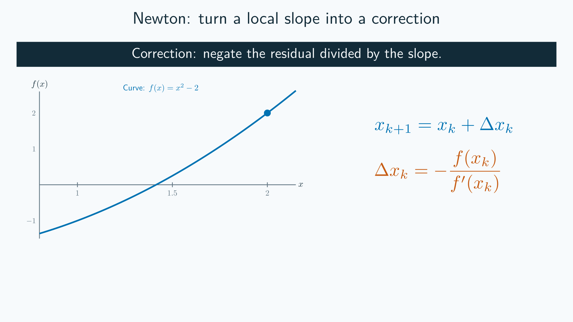
Pause after the first update: why must we reevaluate the curve? Replay, then compare corrections. Explanation.
The next step needs a new tangent
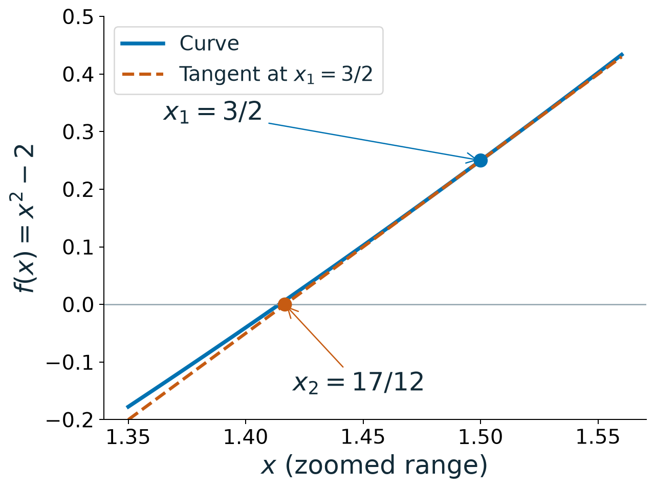
Put our derivative approximation into Newton
When a derivative routine is unavailable, Part I supplies
Replace the derivative in Newton’s update:
We choose h=0 and evaluate an extra nearby sample f(xk+h). The slope estimate must be usable and nonzero; truncation and rounding affect it.
Next idea: we already know the previous iterate’s function value. Can we reuse it instead?
Secant obtains its slope from the iteration
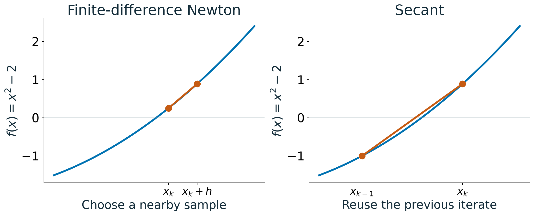
Finite-difference Newton: choose a new sample near the current iterate.
Secant: reuse the previous iterate and its function value. The separation changes with the iteration; there is no separately prescribed h.
Secant reuses two iterates
Approximate Newton’s derivative using two previous points:
Substitute into Newton’s step:
A secant line joins two samples. The secant method specifically reuses successive iterates; their separation replaces a separately chosen h.
Predict the secant intersection
For f(x)=x2−2, start with x0=1 and x1=2.
Use the update to find x2. Which two points will define the following line?
Watch which two values secant keeps
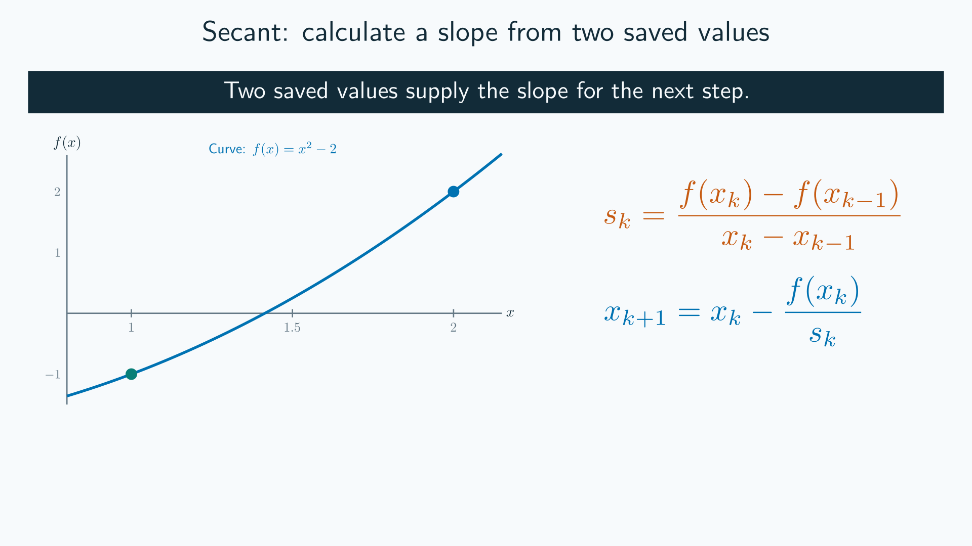
Pause after the first update: which point is retained, and which is discarded? Replay to check. Explanation.
Translate the geometry into an update
For the two points (1,−1) and (2,2), the slope is
The line through the newest point is ℓ(x)=2+3(x−2). Set ℓ(x)=0: x2=4/3.
Now evaluate f(4/3) and retain the previous value f(2) for the next line. Only one new function value is needed. Unlike bisection, we keep recent points rather than opposite signs.
Compare what must be evaluated
| Method | Starting information | New information per ordinary step |
|---|---|---|
| Bisection | Two endpoint values | One midpoint value |
| Newton | One starting point | Function and derivative |
| Secant | Two starting values | One new function value, reusing the previous value |
Count actual evaluations: derivatives may be cheap or expensive.
Distinct inputs can have equal function values
For f(x)=x2−2, choose x0=−1 and x1=1:
The secant is horizontal at y=−1: it never crosses zero. The update divides by zero.
A tiny value difference can also produce an unreliable step. Report the failure; an arbitrary perturbation is not a guaranteed repair.
III · Decide what convergence means
Question: small in which quantity, and relative to which scale?
In Lecture 5, atol and rtol expressed a comparison allowance.
Here we must also decide what evidence to compare with that allowance.
A root-error bound, a small update, and a small residual answer different questions. A solver’s stopping rule belongs in its documented interface.
Three different meanings of small
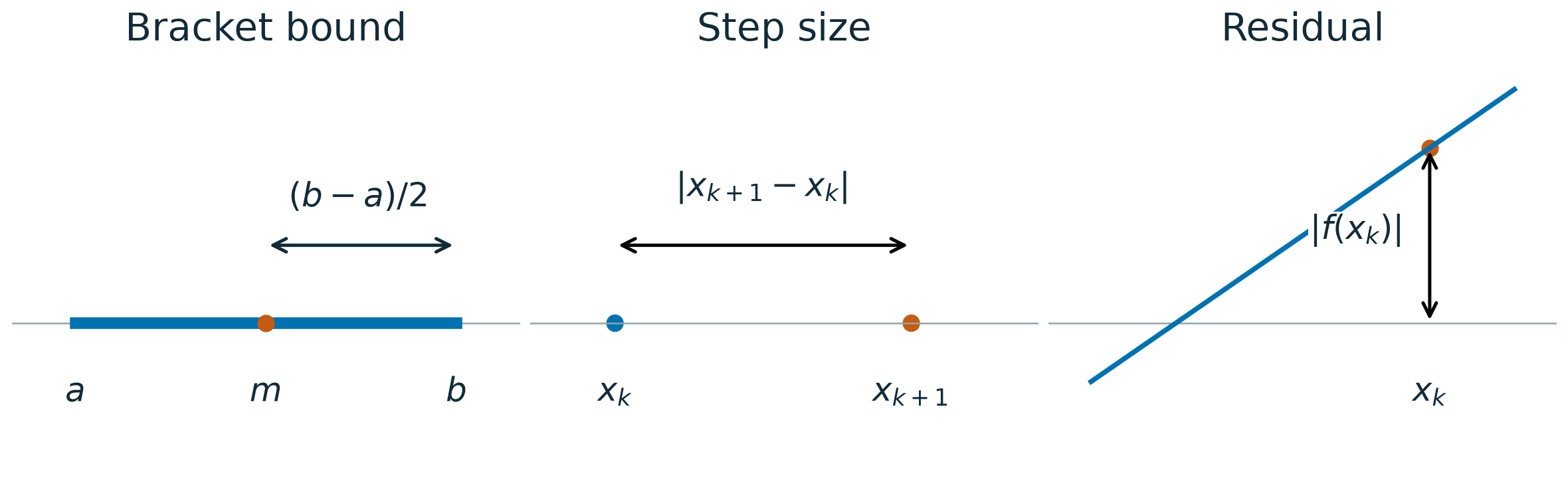
Bound: limits root error for a valid bracket. Step: measures movement. Residual: measures how well the equation is satisfied.
Root error and step have x’s units; residual has f’s units.
A small residual need not locate the root
A simple root has f(r)=0 and f′(r)=0. Near it, Taylor gives
For a stated function-error scale, dividing by a small slope amplifies position uncertainty. This is a local approximation, not a global error bound.
Predict: for f(x)=10−12(x−1) at x=2, what are the residual and root error?
Scaling the function changes the residual
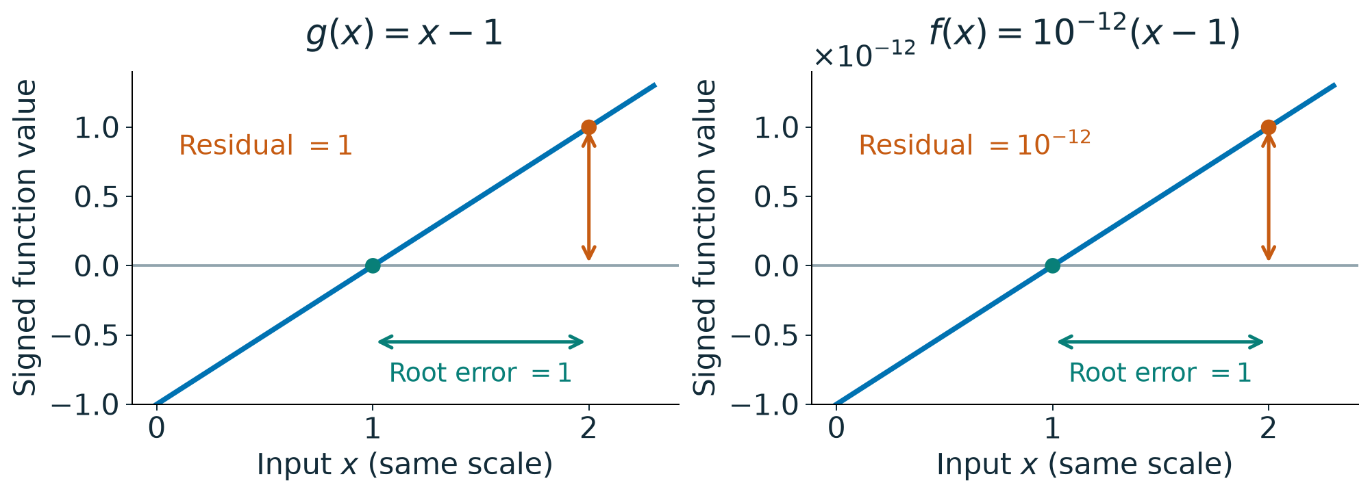
Same input scale; different vertical scales. All quantities here are dimensionless.
Same root, different residual. Choose residual tolerances using the equation’s scale and units.
Give tolerances a meaning
A root-location criterion can use
atol: an absolute allowance in the units of x.rtol: a dimensionless relative allowance.Near zero, a nonzero absolute scale may be necessary.
Bisection compares a bound with τx. Newton and secant compare their step, then inspect the residual separately. A tiny step can also mean stagnation.
In this lab, use the current evaluated midpoint m: compare its bracket bound with τm.
Work out the allowance before running the solver
Suppose x is measured in seconds. Choose, for illustration, atol=10−6s and rtol=10−6.
| Current estimate | τx=atol+rtol∣x∣ |
|---|---|
| x=0 | 10−6s |
| x=1s | 2×10⁻⁶s |
| x=106s | 1.000001s |
The same relative allowance permits a larger absolute difference at larger scales. Choose these values from the task’s accuracy needs; the example is not a universal default.
Predict: does the smaller bracket certify the old midpoint?
For f(x)=x−0.9 on [0,1], take atol=0.25 and rtol=0.
The evaluated midpoint is m=0.5. Its negative value retains the bracket [0.5,1], whose half-width is 0.25.
Predict: can we now return the already evaluated m=0.5 with a root-error bound of 0.25?
Which point is the center of the new bracket?
A bound belongs to a particular midpoint
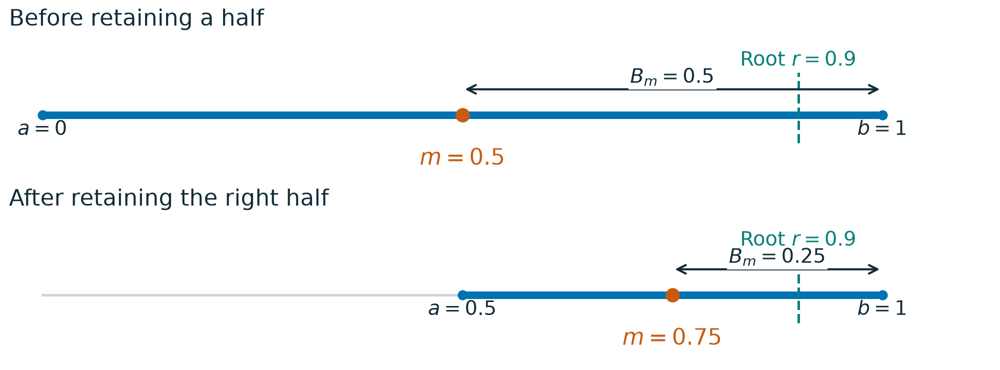
Old midpoint: error 0.4>0.25. New midpoint: error 0.15≤0.25.
Here the root is known. A general solver uses the current bracket bound to certify its midpoint.
IV · Build and test a root-finding module
Work from a mathematical invariant to an interface, then test both success and failure.
Core: implement and test bisection on a non-project equation.
Extension: add Newton or secant and compare iteration histories.
This module can carry into Project 3 when it is posted next week. Today does not introduce a separate graded submission.
Give the code an importable home
root-lab/
├── roots.py
├── tests/
│   └── test_roots.py
└── exploration.ipynb
tests/ → imports → roots.py
Checks behavior and expected failures.
Notebook → imports → roots.py
Plots histories and interprets results.
Keep plots and demonstration runs out of the module’s top level.
Trace → implement → harden
| Stage | Work | Completion check |
|---|---|---|
| Trace | Follow three brackets on paper | Explain retained signs and the current midpoint bound |
| Implement | Build the loop and record midpoints | Known-root and endpoint-root tests pass |
| Harden | Complete input checks and failure tests | Invalid inputs fail; tolerance and iteration limits behave as documented |
Keep the required contract open while working. A first successful root is a checkpoint; complete all three stages before Newton or secant.
Trace first: explain each decision
Use f(x)=x2−2 on [1,2]. Before coding, make three rows:
For each row, explain why the retained endpoints still have opposite signs. The bound belongs to the midpoint evaluated in that row.
Check: a partner can reconstruct your next bracket from your recorded evidence.
Implement: agree on the interface before the loop
def bisect(f, a, b, atol=1e-12, rtol=0.0, max_iter=200):
    """Return (root, n_iter, history); implement the method yourself."""
    raise NotImplementedError
History: evaluated midpoints, in order.
Count: n_iter == len(history).
Return: the last evaluated midpoint, history[-1].
Endpoint zero: return that endpoint with n_iter=0 and history=[].
Required lab contract: inputs and failures
Endpoints: finite real scalars with a<b; handle endpoint zeros before the sign test.
Tolerances: finite, nonnegative; at least one positive.
max_iter: a positive integer, excluding Boolean values.Function values: finite real scalars; compare signs directly rather than multiplying values.
Use ValueError for invalid inputs, an invalid bracket, or unusable function values. Use RuntimeError for an exhausted iteration budget or an unmet tolerance when no interior midpoint is representable.
Continuity and reliable function signs are mathematical preconditions; input checks cannot establish them.
Required lab contract: stopping and recorded evidence
At the evaluated midpoint m of the current bracket [a,b], use
For an exact midpoint, Bm=(b−a)/2. The maximum distance also covers a rounded, off-center midpoint.
Accept a zero computed residual or Bm≤τm; record this midpoint before returning.
Otherwise retain the sign-changing half and continue. Its new width does not certify the old midpoint.
If evaluation underflows to zero or signs are unreliable, the numerical bracket is not a real-arithmetic guarantee.
Record evaluated midpoints only. Endpoint roots have an empty history.
Translate the reading interface deliberately
| Choice | Reading | Lab |
|---|---|---|
| Function | bisection | bisect |
| Tolerance | Absolute tol | atol + rtol*abs(m) |
| Return | Root estimate | (root, n_iter, history) |
Both use a bracket-based position criterion. The lab also records evidence for inspection.
Shared exceptions: ValueError for invalid inputs; RuntimeError for non-convergence.
Reading and lab: evaluation conventions
Reading: may accept the width before evaluating the midpoint. Allows a=b for an endpoint root.
Lab: requires a<b. Evaluate and record the accepted midpoint so root == history[-1].
Endpoint exception: return the endpoint with zero midpoint evaluations and an empty history.
Use the lab contract when writing your tests.
Implement the invariant, not just the update
Check inputs and endpoint roots; establish a valid bracket.
Evaluate its midpoint and record it.
Check a zero computed residual or the current midpoint error bound.
Otherwise retain the half with opposite endpoint signs.
Stop with a useful failure message if the iteration budget is exhausted.
Work on continuous functions. Input checks cannot prove continuity. Do not silently replace a missing bracket with a guessed interval.
Test a known root without solving the project
import numpy as np
from roots import bisect

def test_known_root():
    root, n_iter, history = bisect(
        lambda x: x*x - 2, 1.0, 2.0, atol=1e-8, rtol=0.0
    )
    assert abs(root - np.sqrt(2)) <= 1e-8
    assert n_iter == len(history)
    assert history[-1] == root
A lambda is a small anonymous function. Here it supplies the residual.
Run from the lab directory with python -m pytest.
An expected failure is a passing test
import pytest
from roots import bisect

def test_invalid_bracket():
    with pytest.raises(ValueError):
        bisect(lambda x: x*x + 1, -1.0, 1.0)
pytest.raises passes only if the enclosed call raises the expected exception. Returning a number here is a failure of the solver’s contract.
Save: tests/test_roots.py. Run from root-lab/: python -m pytest.
After module edits, restart the notebook kernel and rerun imports.
Harden: test the contract beyond one root
Use the input and failure contract as your checklist:
Reject invalid endpoints, tolerances, iteration limits, and unusable function values.
Distinguish a missing bracket from exhausted iterations or numerical stagnation.
Check endpoint history and the midpoint to which the bound belongs.
Check: each rejection has an expected exception test. Exercise the relative tolerance before adding another method.
Add tests that could expose a mistake
| Case | Evidence to check |
|---|---|
| x2−2 on [1,2] | Root agrees with 2 within the stated absolute target |
| x−1 on [1,2] | Endpoint root: zero midpoint evaluations and empty history |
x−0.9 on [0,1], atol=0.25, rtol=0 | Return 0.75 after two midpoint evaluations, not 0.5 |
| x2+1 on [−1,1] | ValueError: no sign-changing bracket |
| x2−2, one iteration, tight tolerance | RuntimeError: insufficient iterations |
Trace three brackets on paper; compare signs and widths with your code. Checking only the final root misses invariant failures.
Test the relative term
Design a case where a nonzero rtol changes midpoint acceptance.
Hold the function, bracket, and
atolfixed; compare withrtol=0.Predict which run should stop first, then compare the histories.
Explain why tests using only
rtol=0cannot detect an ignored relative term.
Extend only after bisection is hardened
After the required contract checks pass, add Newton or secant for the same equation.
Plot ∣xk−2∣ against iteration number.
Count function and derivative evaluations separately.
Try a second starting point; explain changed behavior.
A faster example is not a universal ranking. Next lecture develops convergence conditions, failure modes, and safeguards.
Build, test, and explain your module
Need a refresher? Use bisection’s mathematical foundation, module boundaries, and documentation and tests. Build from the invariant before comparing with the reading’s implementation; use today’s interface. Advanced root-finding sections are Lecture 9/reference.
Show your paper trace, passing behavior tests, and required failure checks. Explain what the stopping evidence establishes. Finish hardening bisection before starting an extension.
Keep your module and iteration evidence for Project 3. We continue root finding in Lecture 9; the scientific project is posted next week.
V · Reference for Lecture 9 and the lab
Keep the following material accessible for review and Lecture 9. The required lab contract is in the activity section above.
A derivative from two nearby values
For sufficiently smooth f, Taylor expansion gives
Subtract f(x) and divide by h=0:
The leading truncation error is first order when f′′(x)=0.
Static companion: the first secant
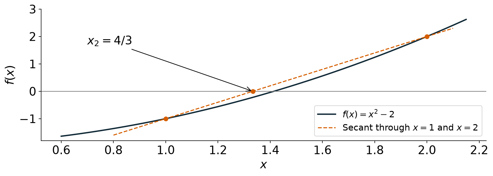
x2=4/3. Next use x1=2 and x2=4/3.
Stop or report failure?
| Evidence | Response |
|---|---|
| Zero computed residual | Return the sampled zero; distinguish computed from exact zero |
| Valid bracket sufficiently narrow | Return its midpoint |
| Small Newton/secant step | Inspect residual and stagnation |
| Invalid bracket, slope, or function value | Report the cause |
| Iteration limit; criterion unmet | Report non-convergence |
A solver should not disguise failure as an ordinary root.
Keep the model; add safeguards
Question: can we combine a fast proposal with a reliable fallback?
Bisection supplies interval evidence. Newton and secant supply model-based proposals. Practical methods can use both.
This is an overview: identify the ingredients today. We will examine convergence and failure behavior in the next lectures.
Advanced methods combine useful ideas
Safeguarded Newton
Maintain a bracket. Use a Newton proposal when it satisfies the safeguard; otherwise take a reliable bracket-reducing step.
Brent’s method
Combine bisection with secant and inverse-quadratic interpolation proposals.
A maintained bracket and acceptance conditions provide reliability under the method’s assumptions.
The same Taylor idea extends to systems
For several unknowns, F contains one residual per equation. The Jacobian records how each residual responds to each unknown: Jij=∂Fi/∂xj. Then
Choose the step by solving
Solve this linear system for the correction Δx; do not explicitly form an inverse. The scalar Newton step is the one-equation version.
Why this matters for data science
Quantiles are inverse problems
For a continuous, strictly increasing CDF C(x) and 0<q<1, the unique quantile satisfies
A numerical bracket must span the target probability. Discrete CDFs instead need a generalized inverse. We know the desired probability q and seek its input x. Numerical inversion is useful when an explicit inverse is unavailable.
Optimization uses related equations
A differentiable loss has stationary points where ∇L=0.
Newton applied to this equation uses the Hessian, the matrix of second derivatives of L.
A root of the gradient may be a minimum, maximum, or saddle; locating it does not classify it.
Optional run: scale the function, keep the root
Predict the two residuals before running. Here both functions have root 1.
# lecture-example: rescaling
x, root = 2.0, 1.0
for scale in (1.0, 1e-12):
    residual = scale * (x - root)
    print(f"scale={scale:.0e}, residual={residual:.0e}, "
          f"root error={abs(x-root):.0e}")
Prepared output: rescaling
Residuals: 1 and 1e−12. Root error: 1 in both cases.
Interpret: why does scaling the residual leave the root location unchanged?
The reference root is available for this teaching example; a general solver usually cannot calculate its actual error.
When a residual gives a bound
Suppose f is continuously differentiable between x and a root r, and a justified bound satisfies ∣f′∣≥m>0 throughout that interval.
The mean value theorem gives
If the computed residual has error at most η, replace the numerator by ∣f(x)∣+η. A derivative at one point alone is not the required interval bound.
Lecture 9 connects this with root sensitivity and nested numerical calculations.