Project 3 uses roots to find where a radiation spectrum peaks, recover a planet’s position, and locate the start and end of a transit: a planet passing in front of its star and blocking some starlight. This companion explains the physics and geometry behind Parts 2–4 of Project 3. The brief specifies the code, tests, and submissions; this page adds no deliverables.
1. Light and the electromagnetic spectrum¶
Visible light is the small part of electromagnetic radiation our eyes detect. Radio, infrared, ultraviolet, X-rays, and gamma rays are the same kind of radiation at different wavelengths. Wavelength is the distance between successive wave crests; frequency counts cycles per second. A photon is a packet of light energy. In vacuum,
Shorter wavelengths mean higher frequency and more energy per photon. They do not, by themselves, mean a brighter source: brightness also depends on how much radiation arrives. Here denotes light frequency; in the orbit sections the same conventional symbol denotes true anomaly. The units and context distinguish them.
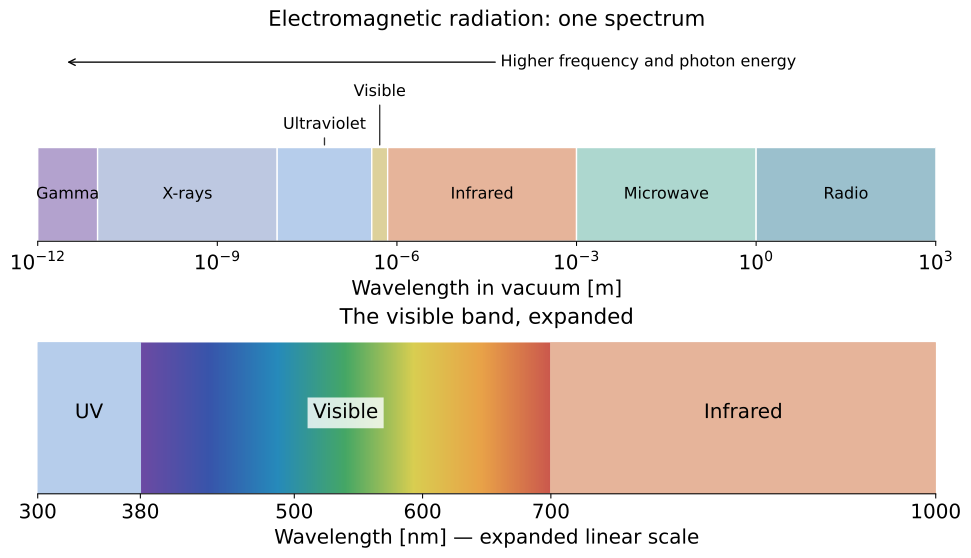
Each tick interval on the upper axis spans a factor of 1000 in wavelength. Visible light occupies only a narrow interval. The lower strip expands it on a linear scale; its colors are illustrative. Band boundaries are conventional, and microwaves are part of the broader radio band. See NASA’s electromagnetic spectrum overview and visible-light guide.
Useful conversions are cm and cm. A peak at nm lies in the visible band; one at nm lies in the infrared. These examples connect the spectrum map to the Planck curves below.
A spectrum is a density¶
Think of a histogram: its bin height can be a count divided by bin width. Likewise, measures radiance in a small wavelength interval. alone is radiance per unit wavelength, not the radiance in the whole spectrum. Radiance describes radiation traveling in a particular direction, per unit apparent emitting area and solid angle. The apparent area is the surface area as viewed from that direction. A solid angle measures the size of a cone of directions; its unit is the steradian (sr). Changing from equal wavelength bins to equal frequency bins changes their widths unevenly because . The density and the location of its maximum can therefore change, while the radiation in corresponding intervals stays the same.
2. Wien’s law: find the wavelength peak¶
A blackbody is an ideal object that absorbs all incident radiation and emits a thermal spectrum determined by its temperature. A spectrum shows how radiation is distributed over wavelength or frequency. Temperature is measured in kelvin (K), an absolute scale with zero at absolute zero. The blackbody’s spectral radiance per unit wavelength is the Planck function:
Here is Planck’s constant, is the speed of light, and is Boltzmann’s constant. CGS means centimeter–gram–second units; the erg is its unit of energy. Use the values in Part 2: in cm and in K. Then has units of energy per time, area, solid angle, and wavelength: .
Wien’s displacement law locates the maximum of this wavelength density:
Doubling the temperature halves the peak wavelength. The spectrum remains broad; the peak does not mean that all photons have that wavelength. Treating a stellar spectrum as a blackbody is an approximation: real spectra include absorption lines and atmospheric effects. Here stellar means relating to a star; absorption lines are narrow dips where material absorbs particular wavelengths, and a stellar atmosphere is a star’s outer gas layers.
The star’s photosphere is the layer from which most of its visible light escapes. A blackbody approximates its thermal radiation. Surface flux is the energy emitted per unit surface area per unit time; luminosity is the total energy emitted by the whole star per unit time. Temperature sets the surface flux, while luminosity also depends on the star’s size.
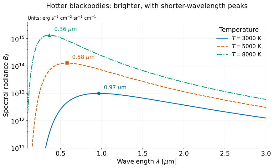
The plot shows the absolute Planck function, with no individual curve normalization. Hotter blackbodies emit more at every wavelength and peak at shorter wavelengths. The logarithmic vertical axis makes the cooler spectrum visible; values below the displayed range are clipped. Markers locate the wavelength peaks. Wavelength is labelled in micrometers ( cm), while radiance remains per cm of wavelength in the CGS units of the equation above. These are ideal blackbody spectra, not measured stellar spectra.
Predict → Play → Explain¶
Before changing temperature, predict how the wavelength peak and emitted surface flux will change. Compare the absolute curves first, then normalize their peaks by dividing each curve by its own maximum. Explain which difference normalization hides. The second view connects the spectral peak to the root-finding problem below.
Derive the equation to solve¶
At fixed , define the dimensionless variable (a ratio with no units)
Logarithmic differentiation keeps the algebra short:
For finite , set this derivative to zero and rearrange:
The positive solution is independent of temperature, giving
This connects Parts 1–2: the generic root finder solves , and the application converts its answer into a physical constant. At fixed temperature, tends to zero at both wavelength extremes. Its unique positive stationary point is therefore the maximum.
Why a zero residual can select the wrong root¶
The rearranged equation also has the root . But the step above assumed : at zero, the denominator vanishes. For finite positive , corresponds to , not a finite-wavelength peak.
The derivative of the root-finding function is
It vanishes at . The function decreases up to that minimum and then increases, crossing zero once more at the desired positive root. This geometry explains both the unwanted zero root and the risk of a large Newton step near a small derivative.
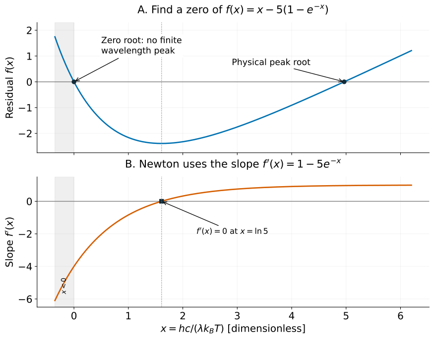
A small residual does not select the physical root. Negative is outside the finite positive wavelength and temperature domain; is its limiting boundary. The dotted line marks a zero derivative, not a root of .
Wavelength and frequency peaks are different¶
Project 2 used , the radiance per unit frequency. Conservation of radiance over corresponding spectral intervals gives
The factor varies with wavelength, so converting the location of the maximum using does not locate the maximum. The underlying radiation is the same; the spectral interval used to define the density changes. See Marr and Wilkin (2012) for a discussion of this distinction.
Integrating the spectrum in Project 2 measures the total emitted flux; finding its peak here measures where the wavelength density is largest. These give Stefan–Boltzmann’s law and Wien’s law, respectively.
3. The model and its coordinates¶
An orbit is a path followed under gravity. Here we track the planet relative to the star. Its path is an ellipse, a closed oval defined by two fixed points called foci (singular: focus): distances from any point on the oval to the two foci add to the same total. The star lies at one focus, away from the ellipse’s center unless the orbit is circular.
Periastron: the point where the planet is closest to the star.
Apastron: the point where it is farthest from the star.
Orbital period : the time for one complete orbit, from one periastron passage to the next. We set at periastron, so measures the elapsed fraction of that time. For example, is a quarter of the period, not a quarter of the distance around the orbit.
Why the planet changes speed¶
Imagine a line joining the star to the moving planet. That line sweeps out a wedge-shaped area. Kepler’s second law says it sweeps equal areas in equal time intervals. During a short time step near periastron, the line is shorter, so a larger sideways step is needed to cover the same area. Near apastron, the line is longer and a smaller step suffices. The planet therefore moves fastest at periastron and slowest at apastron. See NASA’s explanation of Kepler’s laws.
Turn on the figure’s equal-time dots: wider gaps mean greater distance traveled in the same time, hence greater speed. Equal time means equal swept area, not equal distance or equal angle.
To predict a transit, we also need the planet’s apparent position on the sky. The orbital plane contains its path. The sky plane is an imaginary image plane perpendicular to our viewing direction; projecting onto it gives the two-dimensional picture an observer sees.
What the orbital parameters mean¶
Semimajor axis : size. Half the ellipse’s longest width, not the planet’s instantaneous distance from the star.
Eccentricity : shape. Zero gives a circle; larger values below one give more elongated ellipses and a larger difference between closest and farthest distance.
Inclination : tilt. Relative to the sky plane, is face-on (looking directly at the orbit’s face) and is edge-on (looking along its plane). Tilt changes the apparent track and whether it can cross the stellar disk.
Argument of periastron : orientation within the orbital plane. The direction of closest approach, measured from the ascending-node direction. The ascending node is where the planet crosses the sky plane toward the observer. Project 3 fixes .
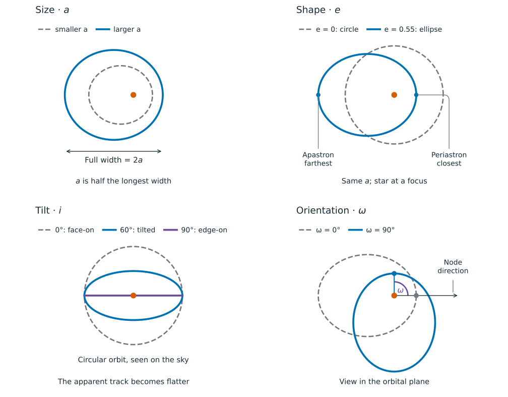
Figure 4:Size, shape, tilt, and orientation. Orange marks the star. The inclination panel shows the observer’s sky; the others show the orbital plane. Dots in the orientation panel mark periastron for two rotations about the stellar focus. View the figure at full size.
In this two-body model, and stay fixed while the planet moves. They orient the orbit; they do not say where the planet is along it. The changing angle supplies that position. Our reference plane is the observer’s sky, with positive toward the observer. We choose along the ascending node. Its direction in the sky plane would otherwise be specified by the node longitude , an angle from a reference direction; choosing this way makes that extra angle unnecessary here.
Watch: tilt, orientation, and position
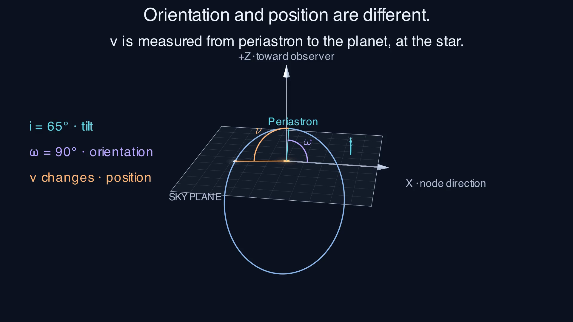
This captioned film uses to make the tilt visible and , the project’s orientation. The required contact cases use . Pause when appears: where does its arc begin, and how is that different from ?
The project model and symbols¶
Treat the star and planet as an isolated Newtonian two-body system: include only their mutual gravity, described by Newton’s laws. Their relative orbit is an ellipse with semimajor axis and eccentricity . The position below is the planet’s displacement relative to the star; the star need not be stationary in an inertial frame, a coordinate frame that is not accelerating or rotating. For the transit, use spherical bodies and a distant observer, so their projected outlines are circles. The stellar disk is the star’s apparent circular face. Project 3 uses uniform brightness across that disk. A light curve plots the received brightness against time.
| Symbol | Meaning |
|---|---|
| , | orbital period and time since periastron, in the same units |
| , | semimajor axis and instantaneous star–planet distance |
| eccentricity; zero gives a circle | |
| , , | mean, eccentric, and true anomaly, in radians |
| angle between the orbital plane and sky plane; is edge-on | |
| argument of periastron, measured in the orbital plane from the ascending node | |
| , | stellar and planetary radii |
| planet-to-star radius ratio | |
| sky-projected center separation divided by |
We fix and put at periastron. In the required edge-on cases, the planet is then directly in front of the star at . For a circular orbit there is no unique periastron; retain this orientation and time origin by convention.
The calculation proceeds as
4. Three angles with different jobs¶
An anomaly is an angular parameter describing position in an orbit. The three anomalies below describe the same instant in different ways; they are linked by the orbit’s geometry, not three angles we choose independently.
We know when we want the planet’s position. On an eccentric orbit, its speed changes, so elapsed time does not translate directly into an angle around the star. Mean anomaly represents the steadily advancing orbital clock. Kepler’s equation, , converts that clock into the geometric parameter . From , we calculate the planet’s distance and its actual direction, the true anomaly . NASA’s orbital-motion explanation describes the same time-to-position sequence.
| Parameter | Question it answers | Where to read it |
|---|---|---|
| Mean anomaly | How much of the period has elapsed? | A clock that advances at a constant rate: |
| Eccentric anomaly | Which auxiliary-circle point maps to the planet? | At ellipse center , from the periastron direction to circle point |
| True anomaly | In which direction is the actual planet? | At star , from periastron toward the planet |
points to , not to the planet. The auxiliary circle is a helper drawing centered at with radius ; there is only one planet. points to the planet from the star. All equations use radians; the figure can display degrees to help read the angles. A radian is an angle unit: one full turn is radians or , and a right angle is radians.
Watch the clock and the planet¶
Reveal Clock & planet → Construct E → Measure ν in order. Scrub time, then turn on equal-time dots. Orbit in space keeps the same instant while you change tilt and orientation. The viewing-angle control moves the diagram’s camera; it does not change the orbit.
One instant, three readings¶
The Film snapshot uses and . Then
| Clock | Construction | Direction | Distance |
|---|---|---|---|
| 0.725 |
Less than 10% of the period has elapsed, yet the planet is already more than from periastron as seen from the star. It moves quickly near periastron, and the star is offset from the ellipse center. Indeed, : the planet has passed to the left of the star even though is still to the right of .
Captioned animation¶
The film has no audio. It builds the construction in stages, then holds time fixed while taking the circular limit. Use the controls to pause or replay it. The static walkthrough below carries the same explanation.
Static walkthrough: time, position, and angles
1. Equal time does not mean equal distance. The clock advances steadily. Every neighboring pair of dots represents the same elapsed time, but the dots crowd together near apastron, where the planet moves more slowly.
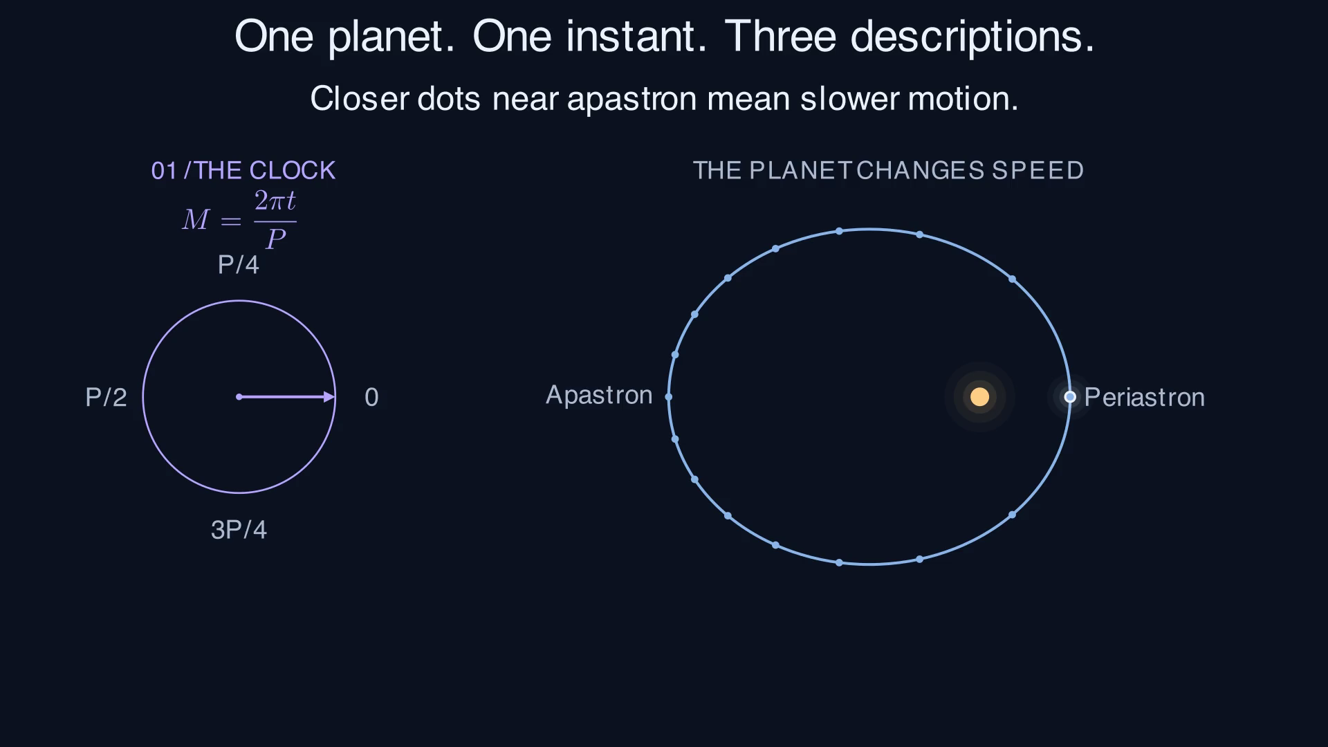
Equal-time sampling for the illustrative orbit. The clock completes one turn while the planet completes one orbit.
2. The angles answer different questions. gives elapsed orbital phase. locates the auxiliary-circle point that maps to the planet. gives the planet’s actual direction from the star.
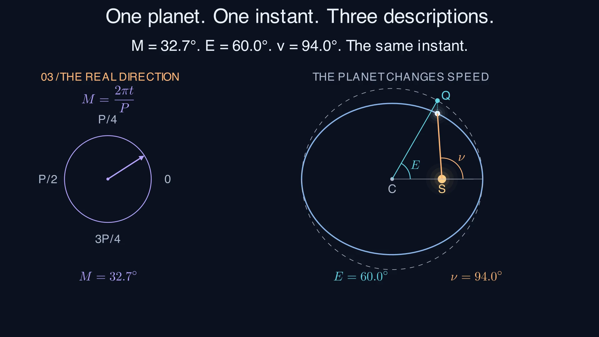
One position, three different angles. is measured using center ; is measured at focus . The separate clock supplies .
Explain: why would moving the planet through equal increments of fail to show equal increments of time when ? Use .
Read the geometry¶
Mean anomaly is a clock:
Here is the clock’s angular rate, in radians per unit time. The clock advances by equal amounts in equal time intervals. For an eccentric orbit, it is not the planet’s physical angle around the star.
Eccentric anomaly parametrizes the ellipse. Draw an auxiliary circle of radius centered on the ellipse’s center . A point at angle on that circle has coordinates . Compress its vertical coordinate by to obtain the planet’s position on the ellipse. The star is at the focus , displaced by from toward periastron. Measured from the star, the orbital-plane coordinates are therefore
True anomaly is the physical angle at the focus: , modulo a full turn.
The distance from the focus is
so . At periastron , ; at apastron , .
The half-angle expression used in the project is
Use a two-argument arctangent to retain quadrant information. Angles differing by describe the same position, but the project’s Kepler solver must return on the same unwrapped branch as its input : keep the count of completed turns rather than reducing every angle to one revolution. For example, corresponds to one full orbit plus the snapshot above, so is near , not just .
5. Why time leads to a root-finding problem¶
Kepler’s second law says the line joining star and planet sweeps equal areas in equal times. Let be the ellipse’s semiminor axis, half its shortest width. From periastron to eccentric anomaly , the swept area is
Compress the auxiliary circle’s sector area by , then subtract the signed triangle area associated with the focus’s offset . The ellipse has area , so equal-area motion gives
Thus measures both the elapsed fraction of a period and the fraction of the ellipse’s area swept from periastron. It does not measure the fraction of the ellipse’s circumference traveled. In the interactive figure, the purple clock sector and orange swept orbital area occupy the same fraction of their respective totals.
For multiple revolutions, interpret area as accumulated swept area. For negative time, use signed area. The same equation remains valid without wrapping the angles.
Given , calculating is direct. Given , we instead solve
For a bound ellipse, , so increases strictly and has one real root for each unwrapped (its limits as have opposite signs). Uniqueness does not guarantee Newton convergence. Near periastron at large , a small derivative can produce a large update.
The residual also needs interpretation. For an approximate solution and exact solution , the mean value theorem gives
This is a bound for the exact mathematical residual. Floating-point evaluation adds round-off error. A small computed residual is useful evidence, but becomes a weaker guarantee of angular accuracy as approaches one.
6. From the orbit to the observer’s sky¶
The orbital radius is a distance in space. For a transit, we need the separation of the two centers on the sky: could the projected disks overlap? Inclination and periastron orientation determine the apparent track. The projected center separation, divided by the stellar radius, is . The Kepler solve supplies position at a trial time; the contact solves find when the projected outlines touch.
Place the star at the origin. Let span the sky plane and let positive point toward the observer. Choose the sky’s axis along the ascending node. With , rotating the orbital plane through inclination gives
Only determine the projected center separation:
At the project’s fixed ,
The final sum of squares avoids subtracting nearly equal numbers near an edge-on mid-transit. At , it reduces to .
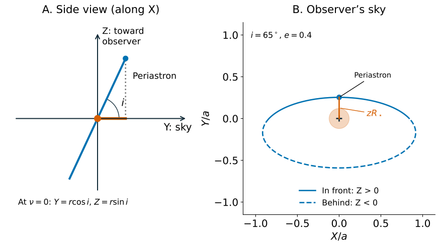
Tilting the orbit changes its sky projection. The illustrative inclination makes the tilt visible. The stellar radius is in the sky view, and the projected track misses the stellar disk. Project 3’s required contact calculations use .
A transit needs both projected overlap and the planet in front: and . Projected overlap with is a secondary eclipse: the star passes in front of the planet and hides some or all of the planet’s light. Because is a distance, it loses this front/back information.
Recover Project 1. In a circular, edge-on orbit, and modulo a full turn. Thus
This is a check of the whole chain: time convention, Kepler solution, angular conversion, and projection. Near , compare absolute errors because a relative error divides by a vanishing reference.
Worked example: one supplied orbital position¶
Take , , , , and a supplied eccentric anomaly radians. This illustrative position is separate from the required edge-on benchmarks. No root solve is needed for this example.
| Step | Calculation | Result |
|---|---|---|
| Orbital position | ; | 0.466025, 0.458258 |
| Distance | 0.653590 | |
| Physical angle | ||
| Sky position | ; | -0.458258, 0.233013 |
| Front/back | +0.403590: toward the observer | |
| Projected separation | 4.112770 |
The planet is on the observer’s side, but it is far from the stellar disk in projection. Being in front is necessary for a transit, not sufficient. Check the rotation by verifying before rounding.
7. Contacts are tangencies between two circles¶
Contact means the apparent planet and star outlines just touch. This is tangency, with the circles touching without crossing at that instant. Scale lengths by : the stellar radius is one, the planetary radius is , and their center separation is . External tangency occurs at the sum of radii, . Internal tangency occurs at their difference, , for .
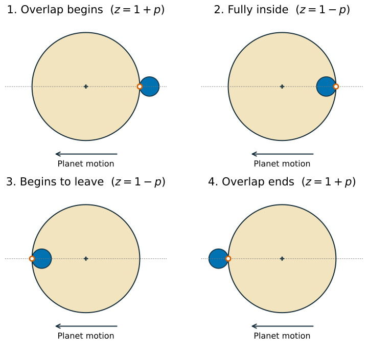
Four distinct contacts for a central transit (a crossing through the star’s apparent center), read left to right across each row. Orange rings mark the tangency points; arrows show planet motion in our sky coordinates. The illustrative planet has .
| Contact | Geometry | What follows |
|---|---|---|
| : | first external tangency | ingress (entry): overlap grows |
| : | first internal tangency | the planet is fully inside the stellar disk |
| : | second internal tangency | egress (exit): overlap shrinks |
| : | second external tangency | overlap has ended |
In a nongrazing transit, the planet’s disk fits fully inside the star’s apparent disk for part of the crossing, so . The two durations are
The second is the full-overlap duration. For a uniformly bright star and an opaque planet (one that does not transmit starlight) with negligible flux of its own, full overlap blocks a fraction of the starlight. Normalized flux divides the received flux by its value outside transit; that baseline is one, and full-overlap flux is . With limb darkening (a stellar disk that looks dimmer toward its edge), the planet crosses regions of different brightness, so this segment need not be flat.
A grazing transit clips the star’s apparent edge without a full-overlap interval. At the boundary where the planet just reaches internal tangency, the two inner contacts merge. Project 3 requires four distinct contacts for its supplied configurations; it asks for a reported failure if that condition is not met elsewhere.
8. Turn the geometry into event equations¶
Define two functions:
Each crosses zero twice during a nongrazing primary transit. At ingress, decreases: the outer crossing comes first, then the inner crossing. At egress the order reverses. Sorting all four times restores chronological order.
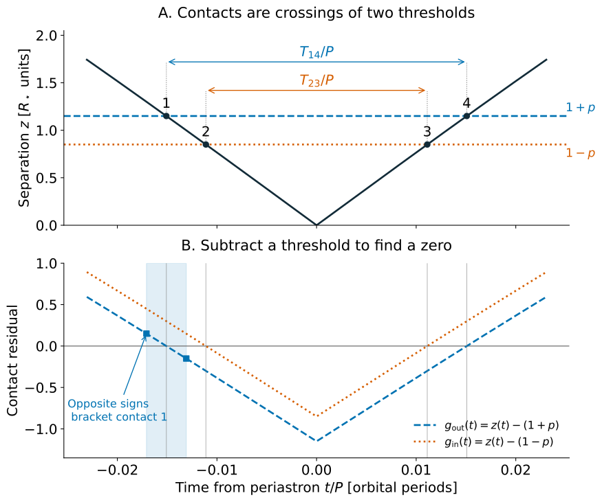
The same event appears as a threshold crossing above and a zero below. Squares mark opposite-sign evaluations that bracket contact 1. The illustrative parameters are , , , and ; they differ from the project’s benchmarks. Time is a fraction of the period.
Use a grid to locate brackets, then refine each crossing with bisection. Compare signs directly, as in the brief; retain exact sampled zeros once. A grid can miss two crossings within one interval, so no detected sign change does not prove there is no transit. Check event selection, refine the grid when needed, and verify the number and order of contacts.
The brief’s window isolates the primary event for its required configurations. It is not a general rule for arbitrary eccentricity, inclination, or periastron orientation. A general event selector also needs the line-of-sight information.
Two numerical solves contribute to the answer¶
Each evaluation of a contact function includes a Kepler solve. An error in changes the computed position and therefore the contact residual. Near a simple crossing, linearization gives the useful sensitivity estimate
A shallow crossing is more sensitive to separation error. This estimate assumes a nonzero slope and sufficiently small errors; it does not apply at a tangency where contacts merge. Bisection bounds a root only when continuity and reliable signs preserve a bracket. Inner-solve errors can shift the contact function or make its signs unreliable near zero.
Finally, both endpoints contribute to duration error:
The required circular-duration comparison checks the full calculation. Optionally, repeat with tighter inner and outer tolerances to see whether the duration stabilizes. A stopping tolerance alone does not establish accuracy.
Why eccentricity changes the duration here¶
At fixed and , the periastron speed is
Our edge-on orientation puts mid-transit at periastron, with velocity in the sky plane. Increasing eccentricity therefore increases the crossing speed near mid-transit, explaining the shorter durations in the project’s cases. Do not generalize this trend to every orientation: a transit near apastron samples a slower part of the orbit. The contact calculation uses the changing position throughout the event, without assuming constant speed.
Further reading¶
Joshua N. Winn, Transits and Occultations, §2, provides a broader treatment of eclipse geometry. Its radius ratio is our , and its true anomaly is our . It chooses the opposite directions for both sky axes; this changes the signs of but leaves unchanged. The figures on this page were generated for this course from the equations shown here.
Model assumptions at a glance¶
| Calculation | Assumption | What the result means |
|---|---|---|
| Wien peak | ideal blackbody; density per wavelength | peak of , not a single emitted color |
| Orbit | isolated Newtonian two-body ellipse | relative star–planet position; no perturbations |
| Transit | distant observer, spherical bodies, uniform stellar brightness | geometric contacts and idealized flux, without limb darkening or noise |
| Temperature zone | equilibrium, full heat redistribution, emissivity one, fixed albedo, no internal heating | temperature bounds, not a climate or habitability prediction |
The eccentricity comparison holds and fixed to isolate the change in orbital shape and speed along the orbit. For the same star and planet masses, fixed fixes through Kepler’s third law; changing does not require changing either. Check the non-intersection condition above before interpreting a mathematical orbit as a physical star–planet system.