Approximation, errors, and quadrature
From continuous mathematics to finite calculations
A computer stores finitely many digits and evaluates finitely many operations. Calculus defines derivatives through limits and integrals through continuous accumulation. Today we connect these descriptions.
The through-line
Jump to: Numbers · Taylor · Tolerances · Quadrature
Represent a number.
Approximate a function locally.
Identify the omitted terms.
Measure an error and choose a comparison tolerance.
Approximate an integral with a sum.
State the approximation before interpreting its numerical error.
Today’s question
How do finite representations and finite approximations affect the calculations we make from continuous mathematics?
By the end of class, you should be able to:
distinguish representation, arithmetic rounding, and truncation;
use a Taylor remainder to explain a leading error term;
explain why a smaller step can hurt a finite difference;
choose
atolandrtolfor a stated comparison; andimplement left-rectangle quadrature and check its first-order prediction.
I · Numbers and operations have finite precision
What changes between a real number on paper and a number stored in a computer?
Goals
distinguish representable values from rounded approximations;
relate absolute spacing to the scale of a number; and
separate representation and arithmetic errors from method truncation.
Predict · which sums are exactly represented?
Python stores these numbers as binary fractions, built from 1/2,1/4,1/8,…. Some fit exactly; others must be rounded.
Predict: will both of these print True?
import numpy as np

print(0.1 + 0.2 == 0.3)
print(0.5 + 0.25 == 0.75)
False
True
== checks exact equality. It does not allow a small discrepancy.
Explain · why False, then True?
Why False?
Just as 1/3=0.3333… repeats in decimal, 0.1 and 0.2 repeat in binary. Python stores rounded approximations.
Adding them and rounding the result produces a slightly different stored
number from entering 0.3 directly:
print(0.1 + 0.2) # 0.30000000000000004
print(0.3) # 0.30.30000000000000004
0.3
== therefore returns False.
Spacing depends on the scale of the number
for value in (1.0, 1.0e8):
spacing = np.spacing(value)
print(f"value={value:.1e}, next-float spacing={spacing:.3e}")
print("binary64 epsilon:", np.finfo(np.float64).eps)value=1.0e+00, next-float spacing=2.220e-16
value=1.0e+08, next-float spacing=1.490e-08
binary64 epsilon: 2.220446049250313e-16
Machine epsilon is the gap from 1.0 to the next larger binary64 number.
It is not a universal absolute error or a guarantee about a calculation.
Explain: why would one fixed absolute tolerance mean different things at scales of 1 and 108?
Three sources of numerical discrepancy
| Source | Example | What we can change |
|---|---|---|
| Representation | Store a decimal fraction in binary | Precision; scaling when appropriate |
| Rounding during arithmetic | Subtract nearly equal approximations | Algebraic formulation; precision |
| Truncation of a mathematical procedure | Replace a derivative by a finite difference | Step size; approximation order |
Measurement uncertainty and model error are additional questions. They are not automatically measured by any of these numerical errors.
An accurate implementation can still calculate an inadequate model.
Reference · finite precision
| Pattern | What it reveals |
|---|---|
np.finfo(np.float64).eps | Spacing immediately above 1 for binary64 |
np.spacing(value) | Local floating-point spacing |
f"{value:.17g}" | More digits than a short default display may show |
np.isfinite(value) | Whether the value is neither infinity nor nan |
Rule: the precision of a representation is not the accuracy of a calculation.
II · Taylor expansion describes a local approximation
How much of a function can we reconstruct from its value and derivatives at one point?
Goals
construct constant, linear, and quadratic local approximations;
interpret the remainder and an order statement;
predict an error ratio under refinement; and
derive a forward difference and explain its rounding tradeoff.
Build the polynomial one derivative at a time
Near x0, write x=x0+h. Taylor’s theorem gives
Each derivative describes another aspect of the local shape.
Constant: the value at the expansion point.
Linear: value and slope.
Quadratic: value, slope, and curvature.
The equality includes Rm+1, the part the polynomial does not capture. Dropping the remainder gives an approximation, f(x0+h)≈Pm(h).
For the remainder formula used here, assume f has continuous derivatives through order m+1 on the interval between x0 and x0+h.
Why these coefficients reproduce the local shape
Start with an unknown polynomial in the displacement h:
Choose its derivatives at h=0 to match those of f at x0:
| Match | Condition | Coefficient |
|---|---|---|
| Value | Pm(0)=f(x0) | a0=f(x0) |
| Slope | Pm′(0)=f′(x0) | a1=f′(x0) |
| Curvature | Pm′′(0)=f′′(x0) | 2a2=f′′(x0) |
| Derivative k≤m | Pm(k)(0)=f(k)(x0) | k!ak=f(k)(x0) |
Why divide by a factorial?
Differentiating hk exactly k times produces k!. That is why the coefficient is f(k)(x0)/k!.
Matching at one point does not make the functions identical everywhere. Taylor’s theorem tells us how to express the remaining difference.
Work out a local model for the exponential
For f(x)=ex at x0=0, every derivative equals 1:
Compare the results: which approximation is best at these offsets? Why does this not guarantee the same accuracy one unit away?
for step in (0.5, 0.1, 0.01):
exact = np.exp(step)
approximations = (1.0, 1.0 + step, 1.0 + step + step**2 / 2)
errors = [abs(exact - value) for value in approximations]
print(f"h={step:.2f}: errors P0, P1, P2 =", np.array(errors))h=0.50: errors P0, P1, P2 = [0.64872127 0.14872127 0.02372127]
h=0.10: errors P0, P1, P2 = [0.10517092 0.00517092 0.00017092]
h=0.01: errors P0, P1, P2 = [1.00501671e-02 5.01670842e-05 1.67084168e-07]
See the value, slope, and curvature
import matplotlib.pyplot as plt
plt.rcParams.update({"font.size": 18})
x_plot = np.linspace(-1.0, 1.0, 401)
fig, ax = plt.subplots(figsize=(9, 4.8), layout="constrained")
ax.plot(x_plot, np.exp(x_plot), color="#122b38", lw=3, label=r"$e^x$")
ax.plot(x_plot, np.ones_like(x_plot), ":", color="#0072B2", lw=2, label=r"$P_0$")
ax.plot(x_plot, 1 + x_plot, "--", color="#D55E00", lw=2, label=r"$P_1$")
ax.plot(x_plot, 1 + x_plot + x_plot**2/2, "-.", color="#009E73", lw=2, label=r"$P_2$")
ax.plot(0, 1, "ko", ms=7)
ax.set(xlabel=r"$x$ (dimensionless)", ylabel="Function value (dimensionless)")
ax.grid(alpha=0.2)
ax.legend(ncol=2)
fig.savefig("lecture-05-taylor.png", dpi=160)
plt.close(fig)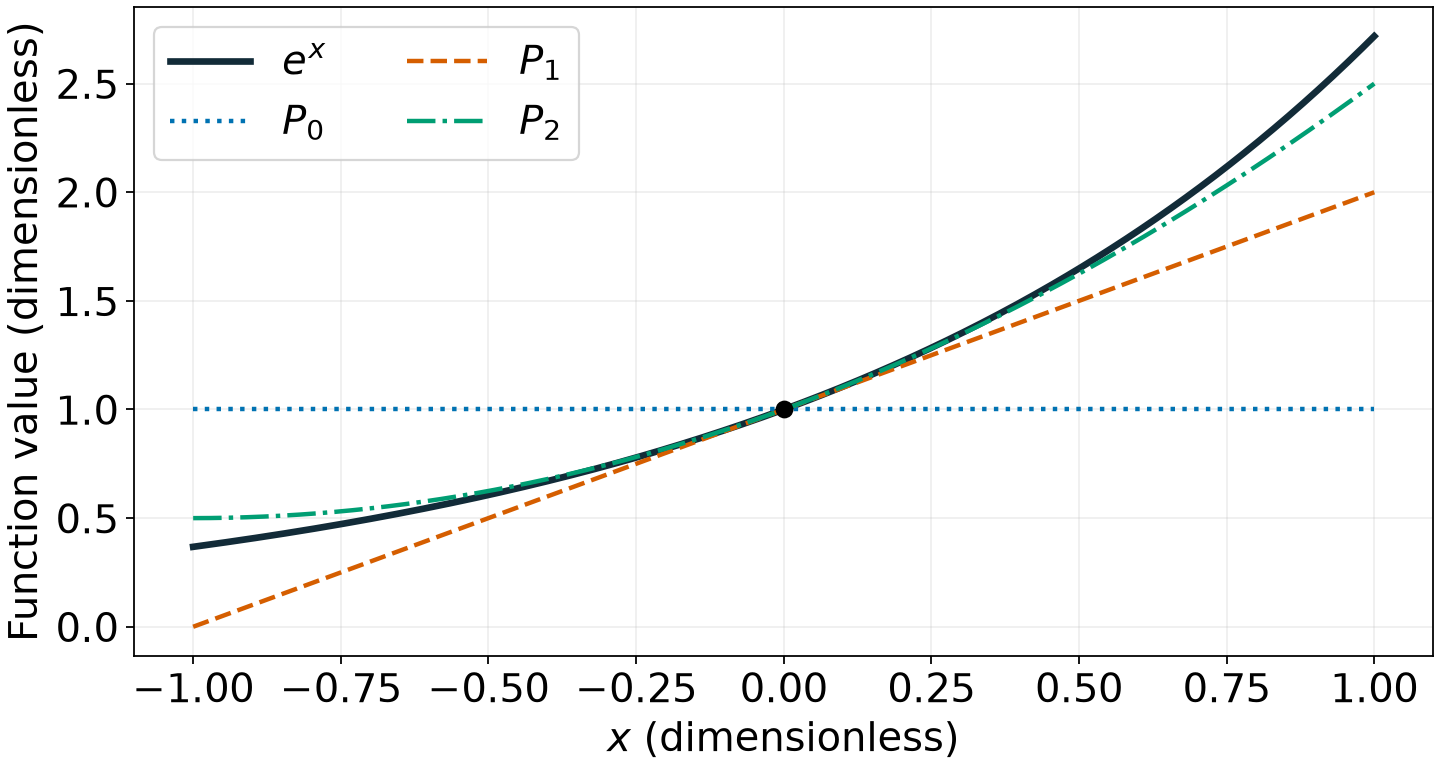
Each polynomial uses information at the same expansion point, x0=0.
Explain: what feature does the quadratic capture that the line cannot?
The remainder tells us what we omitted
For some ξ between x0 and x0+h,
If the derivative is bounded there, the remainder is O(hm+1). This means there is a constant C such that
for sufficiently small h in the stated region.
This is a finite polynomial plus a remainder. We do not need an infinite Taylor series to converge to use this local result.
More terms: accuracy costs arithmetic
For eh with 0≤h≤r, every derivative is bounded by er, so
For a fixed positive h, adding terms reduces the truncation error in this example. Farther from the expansion point, more terms are needed for the same absolute accuracy.
Read the plot · how many terms are enough?
taylor_degrees = np.arange(9)
taylor_cost_errors = {}
fig, ax = plt.subplots(figsize=(9, 4.8), layout="constrained")
for offset, color, marker in ((0.5, "#0072B2", "o"), (2.0, "#D55E00", "s")):
term = total = 1.0
values = [total]
for k in range(1, 9):
term = term * offset / k
total = total + term
values.append(total)
taylor_cost_errors[offset] = np.abs(np.exp(offset) - np.array(values))
ax.semilogy(taylor_degrees, taylor_cost_errors[offset], marker=marker,
color=color, lw=2, label=fr"$h={offset}$")
ax.set(xlabel="Polynomial degree m (m + 1 terms)",
ylabel="Absolute error (dimensionless)", xticks=taylor_degrees)
ax.grid(alpha=0.2, which="both")
ax.legend(title="Distance from expansion point")
fig.savefig("lecture-05-taylor-cost.png", dpi=160)
plt.close(fig)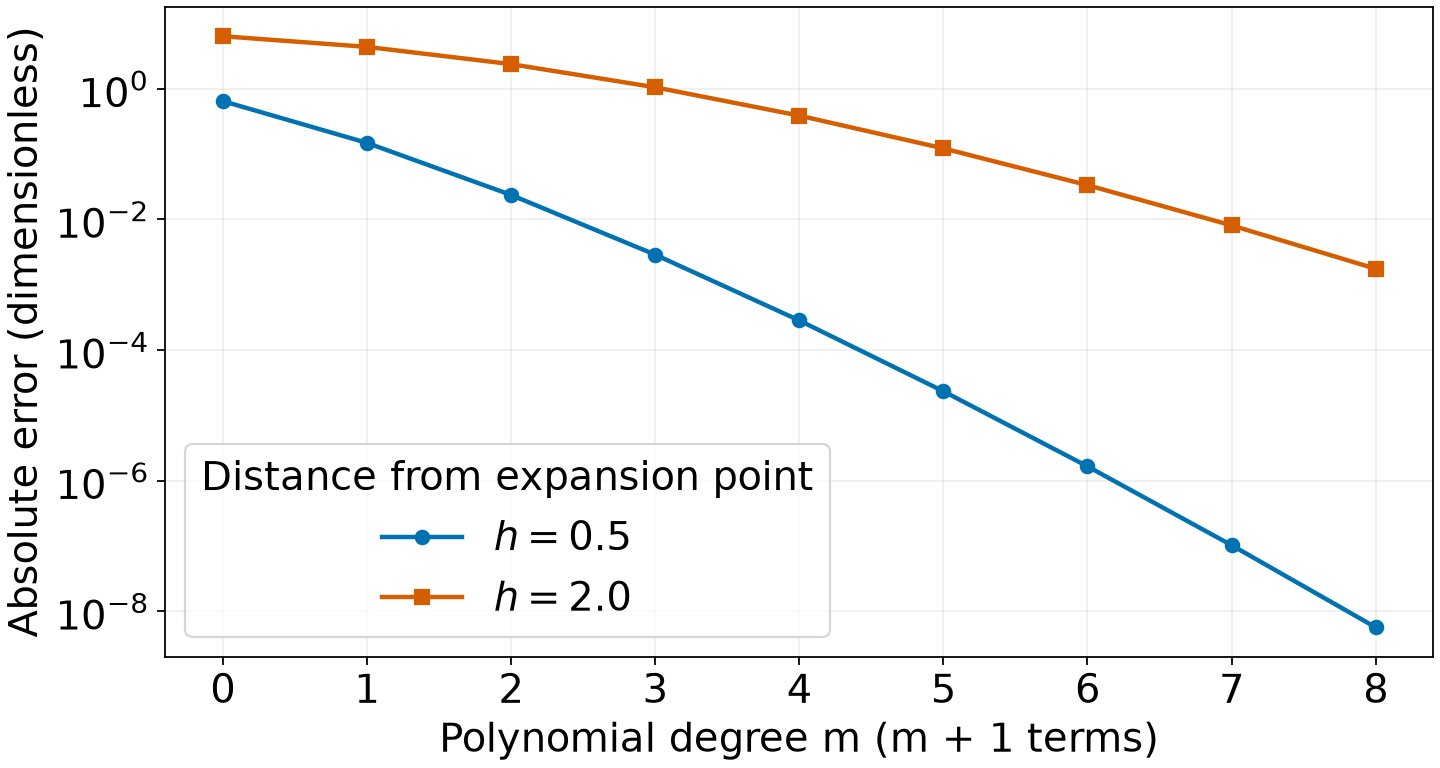
Both approximations use derivatives at zero. More terms improve these results, but evaluating those terms requires additional operations.
Count the work before claiming a speed improvement
For this exponential polynomial, reuse the previous term:
term = total = 1.0 # Start with the constant term, P0 = 1.
for k in range(1, m + 1): # Add terms 1 through m; stop is excluded.
term = term * h / k # One multiplication and one division.
total = total + term # One addition accumulates the next term.Reference · operation count and accuracy
| Degree m | Terms retained | Arithmetic operations in this loop |
|---|---|---|
| 2 | 3 | 6 |
| 4 | 5 | 12 |
| 8 | 9 | 24 |
This counts scalar arithmetic, excluding loop overhead; it is not a timing
measurement. For a general function, obtaining derivatives can add substantial
cost. Library functions such as np.exp use their own optimized algorithms.
Decision: choose enough terms for a justified error target. More terms do not always improve a general function’s approximation at a fixed point, and floating-point rounding can eventually limit improvement even here.
An order predicts a refinement ratio
If the leading error is nonzero and dominates,
| Leading order q | Error after halving h |
|---|---|
| 1 | Approximately one half |
| 2 | Approximately one quarter |
| 4 | Approximately one sixteenth |
An O(hq) bound alone does not establish an exact slope. Cancellation can remove a leading term, and rounding can obscure it.
Apply the rule: if a first-order error is 0.02, what error do you expect after halving h, while the same leading term dominates?
Taylor expansion gives a finite difference
Start with
Subtract f(x) and divide by h=0:
The forward difference has a leading truncation error of order h when f′′(x)=0. We can calculate it without taking a limit in code.
Predict: does this imply that the smallest representable step is best?
Run · smaller steps eventually stop helping
For f(x)=ex at x=0, the exact derivative is 1.
# arange(1, 17) makes the integer array [1, 2, ..., 16]; 17 is excluded.
# Array arithmetic produces all step sizes: 10^-1, 10^-2, ..., 10^-16.
steps = 10.0 ** (-np.arange(1, 17))
# Vectorization: exp, subtraction, and division act element by element.
forward = (np.exp(steps) - 1.0) / steps
# np.abs takes each absolute value: compare every estimate with f'(0) = 1.
derivative_errors = np.abs(forward - 1.0)Read the finite-difference results
# [::3] selects every third entry; zip pairs matching h, estimate, and error.
for step, value, error in zip(steps[::3], forward[::3], derivative_errors[::3]):
print(f"h={step:.0e}: derivative={value:.8f}, error={error:.3e}")h=1e-01: derivative=1.05170918, error=5.171e-02
h=1e-04: derivative=1.00005000, error=5.000e-05
h=1e-07: derivative=1.00000005, error=4.943e-08
h=1e-10: derivative=1.00000008, error=8.274e-08
h=1e-13: derivative=0.99920072, error=7.993e-04
h=1e-16: derivative=0.00000000, error=1.000e+00
Interpret · where does refinement stop helping?
fig, ax = plt.subplots(figsize=(9, 4.8), layout="constrained")
positive = derivative_errors > 0
ax.loglog(steps[positive], derivative_errors[positive], "o-", color="#0072B2", label="Computed absolute error")
ax.loglog(steps, steps/2, "--", color="#D55E00", label=r"Leading truncation term $h/2$")
ax.set(xlabel=r"$h$ (dimensionless)", ylabel="Derivative error (dimensionless)")
ax.grid(alpha=0.2, which="both")
ax.legend()
fig.savefig("lecture-05-difference-error.png", dpi=160)
plt.close(fig)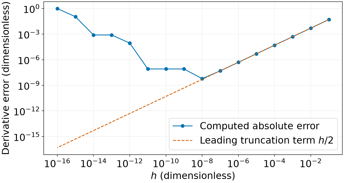
Read toward the left for smaller steps. Exact printed values depend on the floating-point implementation; the truncation prediction does not include rounding.
Why two small errors can produce a larger one
The numerator subtracts values close to 1. Their absolute representation and evaluation errors may be small compared with 1, but large compared with the small difference. Division by h amplifies that discrepancy.
A useful local model for this example is
The constants depend on the function, point, and implementation. This model explains competing trends; it does not give a universal best step size.
For this particular expression, np.expm1(h) / h avoids subtracting 1 from
a rounded exponential. Stable algebra can change the rounding behavior while
leaving the truncation order unchanged.
Reference · Taylor approximation and error order
| Statement | Interpretation |
|---|---|
| f(x0+h)=Pm(h)+Rm+1 | An approximation plus its remainder |
| Rm+1=O(hm+1) | A local bound under the stated smoothness conditions |
| E(h)≈Chq | A dominant, nonzero error term predicts a refinement ratio |
| E(h)/E(h/2)≈2q | An observable to compare with that prediction |
Rule: state the region and assumptions before interpreting an observed order.
III · Measure the error before deciding what is acceptable
What does it mean for a result to agree with a reference closely enough?
Goals
compute absolute and relative discrepancies;
state the units and roles of
atolandrtol;handle a zero or very small reference deliberately; and
justify a tolerance independently of whether a test passes.
Absolute and relative errors answer different questions
For a computed value Q and a reference Q⋆,
Absolute error has the same units as Q.
Relative error is dimensionless; multiply by 100 for percent error.
At a zero reference, relative error is undefined.
Against an approximate reference, these are discrepancies that also contain the reference’s error.
A tolerance is an acceptance criterion. It does not measure or reduce error.
atol and rtol state two scales of agreement
For finite values, NumPy evaluates
np.isclose(computed, reference, rtol=relative_allowance,
atol=absolute_allowance)atol has the quantity’s units. rtol is a fraction: 0.01 means 1%.
Put the reference second: NumPy uses it to set the relative scale.
With both nonzero, NumPy adds the allowances. Agreement need not satisfy each allowance separately.
See the tolerance as an acceptance region
Read the figure: with atol=0.1 cm and rtol=0.1, how much discrepancy is
allowed at a reference of zero? At a reference of 2 cm?
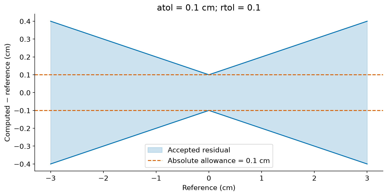
NumPy accepts finite comparisons inside the shaded region, including its boundary.
Interpret the tolerance
At zero: 0.1 cm. At 2 cm: 0.1+0.1(2)=0.3 cm. These tolerances are comparison choices, not floating-point properties.
Explain: does passing this comparison tell us whether a model describes its physical system correctly?
Predict · the same absolute error at different scales
Suppose our stated criterion is relative agreement within one part in a million, with no separate absolute allowance.
reference = np.array([1.0, 1.0e6])
computed = reference + 0.1
rtol = 1.0e-6
atol = 0.0
print("absolute error:", np.abs(computed - reference))
print("allowed error:", atol + rtol * np.abs(reference))
print("accepted:", np.isclose(computed, reference, rtol=rtol, atol=atol))absolute error: [0.1 0.1]
allowed error: [1.e-06 1.e+00]
accepted: [False True]
Predict: which comparisons pass? State the allowed error for each reference.
Results · the same absolute error at different scales
print("absolute error:", np.abs(computed - reference))
print("allowed error:", atol + rtol * np.abs(reference))
print("accepted:", np.isclose(computed, reference, rtol=rtol, atol=atol))absolute error: [0.1 0.1]
allowed error: [1.e-06 1.e+00]
accepted: [False True]
Explain: why does one comparison fail and the other pass? Would changing the tolerance change either computed value?
Near zero, the absolute scale matters
Suppose an example calculation has an independently chosen absolute accuracy target of 10-8 cm. Compare its residual with zero:
residual_cm = 3.0e-9
print("relative only:", np.isclose(residual_cm, 0.0, rtol=0.01, atol=0.0))
print("absolute target:", np.isclose(residual_cm, 0.0, rtol=0.0, atol=1.0e-8))relative only: False
absolute target: True
No finite relative tolerance permits a nonzero discrepancy against exactly
zero when atol=0. Choose an absolute scale from the question being tested.
The 10-8 cm here is a stated example target, not a universal recommendation.
A default absolute tolerance can hide a large relative error
These example fluxes differ by 100% of the reference value:
reference_flux = 1.0e-12 # erg / (s cm^2)
computed_flux = 2.0e-12
print("NumPy defaults:", np.isclose(computed_flux, reference_flux))
print("stated 1% target:", np.isclose(
computed_flux, reference_flux, rtol=0.01, atol=0.0
))NumPy defaults: True
stated 1% target: False
NumPy’s default atol=1e-8 is larger than either value in these units.
Always check the tolerance against the scale and units of the calculation.
Source: NumPy isclose documentation.
Similar comparison functions have different rules
For finite scalar values a and b:
| Function | Permitted discrepancy |
|---|---|
np.isclose(a, b, rtol=r, atol=t) | t+r∣b∣ |
math.isclose(a, b, rel_tol=r, abs_tol=t) | max(t,rmax(∣a∣,∣b∣)) |
Lecture 1 used math.isclose; today we use NumPy for arrays. The formulas
are different, so do not treat a name change as the whole conversion.
np.isclose returns one Boolean per element. np.allclose asks whether
all elementwise comparisons pass. Ensure arrays have the intended shapes
before comparing: NumPy can broadcast them.
Sources: NumPy ·
Python math.isclose.
Choose a tolerance from the claim
Identify the reference and its accuracy.
State the units and whether an absolute or fractional discrepancy matters.
Use a method error bound, a convergence study, or a stated accuracy target.
Set the tolerance before inspecting whether the result passes.
If it fails, investigate the calculation and the criterion.
Check that quantities expected to be finite are finite. A comparison is not a substitute for that contract.
Explain: if a method is first order, does asking for rtol=1e-12 make it
more accurate? What would you actually need to change?
Reference · tolerances and error measurements
| Quantity or choice | Meaning |
|---|---|
abs(computed - reference) | Absolute discrepancy, in the quantity’s units |
Absolute discrepancy divided by abs(reference) | Fractional discrepancy for a nonzero reference |
rtol=0.0 | Only the absolute allowance contributes |
atol=0.0 | Only the relative allowance contributes |
Both nonzero in np.isclose | NumPy adds the absolute and reference-scaled allowances |
Rule: a tolerance expresses a claim. Increasing it does not improve the result.
IV · Quadrature replaces an integral with a finite sum
How can local function approximations give a numerical value for an integral?
Goals
distinguish the interval, panels, nodes, heights, and weights;
implement a callable-based left-rectangle rule;
connect local area error to composite error; and
compare computed errors with a ratio prediction and a bound.
Approximate one panel, then add the areas
Consider a fixed interval [a,b], with a<b. Divide it into n equal panels:
There are n panels and n+1 boundary points.
On panel [xi,xi+1], use the constant approximation f(x)≈f(xi):
Adding the panel contributions gives the left-rectangle rule:
Explain · which area is missing?
For f(x)=sinx on [0,π/2], the function is increasing and the exact integral is 1. Use the rectangles to explain the sign of Ln−1.
fig, ax = plt.subplots(figsize=(9, 4.8), layout="constrained")
panel_count = 6
width = (np.pi/2) / panel_count
left_nodes = width * np.arange(panel_count)
x_plot = np.linspace(0, np.pi/2, 301)
ax.bar(left_nodes, np.sin(left_nodes), width=width, align="edge",
color="#0072B2", alpha=0.25, edgecolor="#0072B2", label="Left rectangles")
ax.plot(x_plot, np.sin(x_plot), color="#122b38", lw=2.5, label=r"$\sin x$")
ax.plot(left_nodes, np.sin(left_nodes), "o", color="#0072B2", label="Sample positions")
ax.set(xlabel=r"$x$ (radians)", ylabel=r"$\sin x$ (dimensionless)", xlim=(0, np.pi/2))
ax.legend()
fig.savefig("lecture-05-rectangles.png", dpi=160)
plt.close(fig)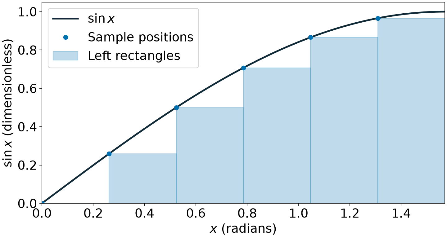
The first rectangle has height zero. That panel still contributes to the integral, which explains part of the underestimate.
Build the nodes before the function
a, b, n = 0.0, np.pi/2, 6
width = (b - a) / n
nodes = a + width * np.arange(n)
heights = np.sin(nodes)
print("panels:", n, "sampled heights:", heights.size)
print("left endpoints:", nodes)
print("rectangle sum:", width * np.sum(heights))panels: 6 sampled heights: 6
left endpoints: [0. 0.26179939 0.52359878 0.78539816 1.04719755 1.30899694]
rectangle sum: 0.8633821943925831
np.arange(n) supplies the integers 0 through n-1. The last sample is
b−h, not b.
Explain: why would np.linspace(a, b, n) give the wrong node spacing here?
One function implements the rule
width = (b - a) / n
nodes = a + width * np.arange(n)
return float(width * np.sum(f(nodes)))Set the panel width.
Sample the left endpoints.
Add height × width.
The complete function on the next slide also validates n.
Contract: finite scalar limits; f accepts and returns finite arrays of matching
shape. n is a positive integer; booleans are excluded.
Reference · rectangle implementation
def rectangle(f, a, b, n):
"""Left rectangles; first-order composite error for smooth f."""
# Reject Boolean values, then require a Python or NumPy integer.
if isinstance(n, (bool, np.bool_)) or not isinstance(n, (int, np.integer)):
raise ValueError("n must be a positive integer")
# A valid integer type can still have an invalid value.
if n <= 0:
raise ValueError("n must be a positive integer")
width = (b - a) / n
nodes = a + width * np.arange(n)
return float(width * np.sum(f(nodes)))
print(rectangle(np.sin, 0.0, np.pi/2, 100))0.9921254566056329
Why use isinstance for input checks?
isinstance(value, type) asks whether a value belongs to a type, including its
subclasses. A tuple of types accepts any of the listed types.
print(isinstance(6, int)) # True
print(isinstance(6.0, int)) # False
integer_types = (int, np.integer)
print(isinstance(np.int64(6), integer_types))
print(isinstance(True, int)) # True: bool is an intTrue
False
True
True
A panel count describes a number of intervals. The rule accepts positive
integers and rejects True, 6.0, and 6.5 under its stated contract.
Silently applying int(n) could turn 6.5 into 6 and change the requested grid.
The first check rejects unsuitable types; n <= 0 rejects unsuitable values.
raise ValueError(...) stops the calculation and tells the caller which
input requirement was violated. This example checks n; finite limits and
finite, matching integrand arrays remain caller preconditions here.
Passing a function is different from calling one
| Expression | What it supplies |
|---|---|
np.sin | A callable: the rule can choose where to evaluate it |
np.sin(nodes) | Values at nodes already chosen |
rectangle(np.sin, a, b, n) | A quadrature calculation using the sine function |
The rule owns the grid. The callable owns the mathematical function.
Predict: what must change inside rectangle to integrate ex instead?
Reuse the rule with another function
Nothing inside rectangle changes. Pass a different callable and interval.
print("sine:", rectangle(np.sin, 0.0, np.pi/2, 100))
print("exponential:", rectangle(np.exp, 0.0, 1.0, 100))
sine: 0.9921254566056329
exponential: 1.7097047383081225
Taylor expansion explains the rectangle error
Within one panel, put x=xi+s with 0≤s≤h:
Integrate each term:
The rectangle retains the first term. Its one-panel error is O(h2). For an increasing function, the missing leading area is positive.
One-panel error and whole-interval error differ
The interval length b−a stays fixed while n=(b−a)/h increases. If panel errors are uniformly bounded by Ch2, their sum is bounded by
Thus the composite left-rectangle rule has an O(h) error bound.
We can replace the unspecified constant C by a bound on the slope. The next slide derives that bound for any continuously differentiable f on [a,b].
Derive a bound for any smooth integrand
Assume a<b and ∣f′(x)∣≤M1 throughout [a,b]. The mean value theorem bounds the change in height inside panel i:
The panel’s signed area error is the integral of that height difference:
Take the absolute value, bound the integrand, and integrate:
The factor 1/2 is the area of a triangle with base h and height M1h.
Sum the panel bounds
Adding the absolute panel bounds gives
These statements concern quadrature error in exact arithmetic. A numerical test must also allow for relevant floating-point effects.
Choose a panel count from an error target
For a requested absolute quadrature error τ>0, it is sufficient that
Choose a positive integer:
The ceiling rounds upward. This gives a sufficient count, not necessarily the smallest count that works: the bound allows the largest slope on every panel and ignores cancellation between panel errors.
This requires a justified derivative bound. Sampling f′ at a few points does not prove that no larger slope occurs between them. Floating-point error is a separate contribution to the total error budget.
Run · test the first-order prediction
previous_error = None
for n in (20, 40, 80, 160):
    estimate = rectangle(np.sin, 0.0, np.pi/2, n)
    error = abs(estimate - 1.0)
    ratio = "—" if previous_error is None else f"{previous_error/error:.3f}"
    print(f"n={n:3d}: estimate={estimate:.7f}, error={error:.3e}, ratio={ratio}")
    previous_error = error
n= 20: estimate=0.9602160, error=3.978e-02, ratio=—
n= 40: estimate=0.9802365, error=1.976e-02, ratio=2.013
n= 80: estimate=0.9901504, error=9.850e-03, ratio=2.007
n=160: estimate=0.9950832, error=4.917e-03, ratio=2.003
Compare En/E2n with 2. One accurate answer would not show this pattern.
Explain: why would changing the integrand change the error magnitude even if the leading order stayed the same?
Use the error bound to choose an absolute tolerance
For sine on [0,π/2], f′(x)=cosx, so M1=1 and b−a=π/2:
At n=100,
Check the sine estimate against its bound
n = 100
error_bound = np.pi**2 / (8*n)
estimate = rectangle(np.sin, 0.0, np.pi/2, n)
print("observed error:", abs(estimate - 1.0))
print("theoretical bound:", error_bound)
print("within bound:", np.isclose(estimate, 1.0, rtol=0.0, atol=error_bound))
observed error: 0.007874543394367106
theoretical bound: 0.012337005501361697
within bound: True
The measured error is below the bound; rounding is much smaller here. Passing checks this example, not the general theorem.
Compute a sufficient panel count
# Choose n to make the quadrature bound at most 0.01.
target = 0.01
required_n = max(1, int(np.ceil(np.pi**2 / (8*target))))
print("sufficient panels for target 0.01:", required_n)  # 124 panels.
sufficient panels for target 0.01: 124
The ceiling rounds upward: 124 panels suffice for this quadrature bound.
Reference · left-rectangle quadrature
| Component | Expression |
|---|---|
| Panel width | width = (b - a) / n |
| Left endpoints | nodes = a + width * np.arange(n) |
| Heights | f(nodes) |
| Weighted sum | width * np.sum(f(nodes)) |
| Expected leading composite order | 1 for a nonvanishing leading term and a smooth integrand |
Rule: the integrator selects the grid; the callable supplies the function values.
Same panels, different rectangle heights
Keep h=(b−a)/n and the same panel boundaries. Change only where each height is sampled, with i=0,…,n−1:
| Rule | Sample location | Composite sum |
|---|---|---|
| Left | a+ih | Ln=h∑if(a+ih) |
| Right | a+(i+1)h | Rn=h∑if(a+(i+1)h) |
| Midpoint | a+(i+21)h | Mn=h∑if(a+(i+21)h) |
Compare left, right, and midpoint rectangles
variant_n = 6
variant_h = (np.pi/2) / variant_n
panel_left = variant_h * np.arange(variant_n)
curve_x = np.linspace(0, np.pi/2, 301)
rectangle_variants = {}
fig, axes = plt.subplots(1, 3, figsize=(12, 4.4), sharey=True, layout="constrained")
for ax, name, shift, color, marker in zip(
    axes, ("Left", "Right", "Midpoint"), (0.0, 1.0, 0.5),
    ("#0072B2", "#D55E00", "#009E73"), ("o", "s", "^")
):
    sample_x = panel_left + shift * variant_h
    heights = np.sin(sample_x)
    rectangle_variants[name] = float(variant_h * np.sum(heights))
    ax.bar(panel_left, heights, width=variant_h, align="edge", color=color,
           alpha=0.25, edgecolor=color)
    ax.plot(curve_x, np.sin(curve_x), color="#122b38", lw=2)
    ax.plot(sample_x, heights, marker, color=color, ms=6)
    ax.set(title=f"{name}: {rectangle_variants[name]:.4f}",
           xlabel=r"$x$ (radians)", xlim=(0, np.pi/2))
axes[0].set_ylabel(r"$\sin x$ (dimensionless)")
fig.savefig("lecture-05-rectangle-variants.png", dpi=160)
plt.close(fig)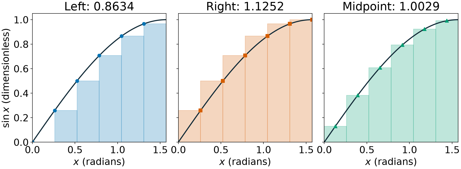
All three rules use six heights. The rectangles retain the same bases; moving the sample changes their heights and the estimated area.
What changes when we move the sample?
For an increasing function and a<b,
The sum in the difference telescopes: interior samples cancel, leaving only the endpoint values. For a decreasing function, the inequalities reverse.
Predict · which side is the midpoint area on?
The midpoint rule cancels the linear contribution about each panel’s center, so its composite error is O(h2) when the second derivative is bounded. It need not lie on the same side of the integral as the left rule.
Predict: sine is concave down on this interval. Does midpoint sampling underestimate or overestimate its area?
Explain the midpoint estimate
A tangent at each midpoint lies above the curve, and its integral over the symmetric panel equals the midpoint rectangle area: here the midpoint rule overestimates.
Next lecture, connecting endpoint heights gives trapezoids. In fact, Tn=(Ln+Rn)/2 on this uniform grid. We will derive why that average also improves the order.
Documentation for the next question
| Resource | Use it for |
|---|---|
NumPy finfo | Floating-point representation limits |
NumPy isclose | Exact tolerance semantics |
NumPy expm1 | Stable evaluation near zero |
Python isinstance | Type checks, tuples of types, and subclasses |
NumPy arange and abs | Array indices and elementwise absolute values |
Use the course readings for derivations and worked examples. Use official API documentation to check parameter meanings, assumptions, and return values.
When a comparison surprises you, print the discrepancy and the allowed discrepancy before changing either tolerance.
Exit check
What is the difference between truncation error and rounding error?
Why can reducing h hurt a forward difference?
Against a zero reference, which tolerance sets the allowed discrepancy?
Why is a one-panel O(h2) error consistent with a composite O(h) error?
What should happen to a first-order error when the panel count doubles?
Use the mechanism in each answer, not only the name of the error.
Carry forward
Next class: replace each constant panel approximation with a line, then a
quadratic. We will organize the rectangle rule in a module and test it on
sinx using pytest.
Project 2 uses these ideas to build and assess numerical integrators. The assignment brief specifies the deliverables; today’s rule and error comparison give you a starting point.
Reading guide in Numerical Methods: Foundations, Part 1, “Forward Difference”; Part 2, the absolute/relative error and tolerance discussions; Part 3, “Taylor polynomial and remainder.” In Roots and Quadrature, Part 2, review the rectangle-rule section. The longer chapters are references; the other methods are not preparation for today’s rectangle implementation.