Trapezoids, Simpson, modules, and tests
Improve a local approximation, then make its implementation reusable
Last class we replaced the function on each panel with a constant. Today we use a line and a quadratic, then organize and test the rectangle rule in a lab.
The through-line
Jump to: Trapezoid · Simpson · Modules and tests · Sine lab
Approximate the function on one panel.
Integrate that approximation.
Assemble a composite rule and explain its error order.
Put a reusable function in a module.
Write a test whose reference and tolerance have a stated basis.
The same choices apply to many scientific integrands.
Today’s question
How do better local approximations lead to better quadrature rules, and how can we make those rules reusable and testable?
By the end of class, you should be able to:
derive trapezoid and Simpson weights from local polynomials;
explain their composite orders and smoothness conditions;
organize a numerical function in an importable module;
run
pytesttests from the project root; andjustify an accuracy assertion and test invalid inputs.
Recall · what a left rectangle retains
On a panel of width h,
The left rectangle keeps hf(xi) and omits the slope contribution.
Predict: if we use both endpoint heights and join them with a line, which term can we capture? What kind of function would the new rule integrate exactly?
I · Trapezoids retain the local slope
What accuracy do we gain by connecting the two endpoint heights?
Goals
integrate a linear interpolant on one panel;
assemble the endpoint and interior weights; and
derive the local and composite error orders with Taylor expansion.
Integrate the line between the endpoints
With s=x−xi on 0≤s≤h, the interpolating line is
Its area is
This is the trapezoidal rule on one panel. A linear function is reproduced exactly by its endpoint interpolant.
Interior nodes belong to two neighboring trapezoids
Adding the panel contributions gives
| Node | Number of neighboring panels | Composite weight |
|---|---|---|
| x0 | 1 | h/2 |
| x1,…,xn−1 | 2 | h |
| xn | 1 | h/2 |
There are n panels and n+1 sampled heights. The weights carry the units of the integration variable.
Taylor expansion identifies the trapezoid error
Expand around the left endpoint:
whereas the exact panel integral is
Therefore Ti−Ii=12h3fi′′+O(h4). The local error is O(h3); summing over a fixed interval gives O(h2).
Predict: sine is concave down on [0,π/2]. Does the chord lie above or below the curve, and what sign should Tn−I have?
Compare the local approximations
import numpy as np
import matplotlib.pyplot as plt

plt.rcParams.update({"font.size": 18})
x = np.linspace(0.0, 1.0, 301)
# The quadratic interpolates exp(x) at 0, 1/2, and 1.
quadratic = (2*(x-0.5)*(x-1)
             - 4*np.exp(0.5)*x*(x-1) + 2*np.exp(1)*x*(x-0.5))
approximations = (np.ones_like(x), 1+(np.e-1)*x, quadratic)
fig, axes = plt.subplots(1, 3, figsize=(12, 4.5), sharey=True, layout="constrained")
for ax, approximation, title in zip(axes, approximations, ("Constant", "Linear", "Quadratic")):
    ax.plot(x, np.exp(x), color="#122b38", lw=2.5, label=r"$e^x$")
    ax.plot(x, approximation, "--", color="#D55E00", lw=2, label="Interpolant")
    ax.fill_between(x, approximation, alpha=0.15, color="#0072B2")
    ax.set(title=title, xlabel=r"$x$ (dimensionless)")
    ax.grid(alpha=0.2)
axes[0].set_ylabel("Function value (dimensionless)")
axes[0].legend(fontsize=11)
fig.savefig("lecture-06-interpolants.png", dpi=160)
plt.close(fig)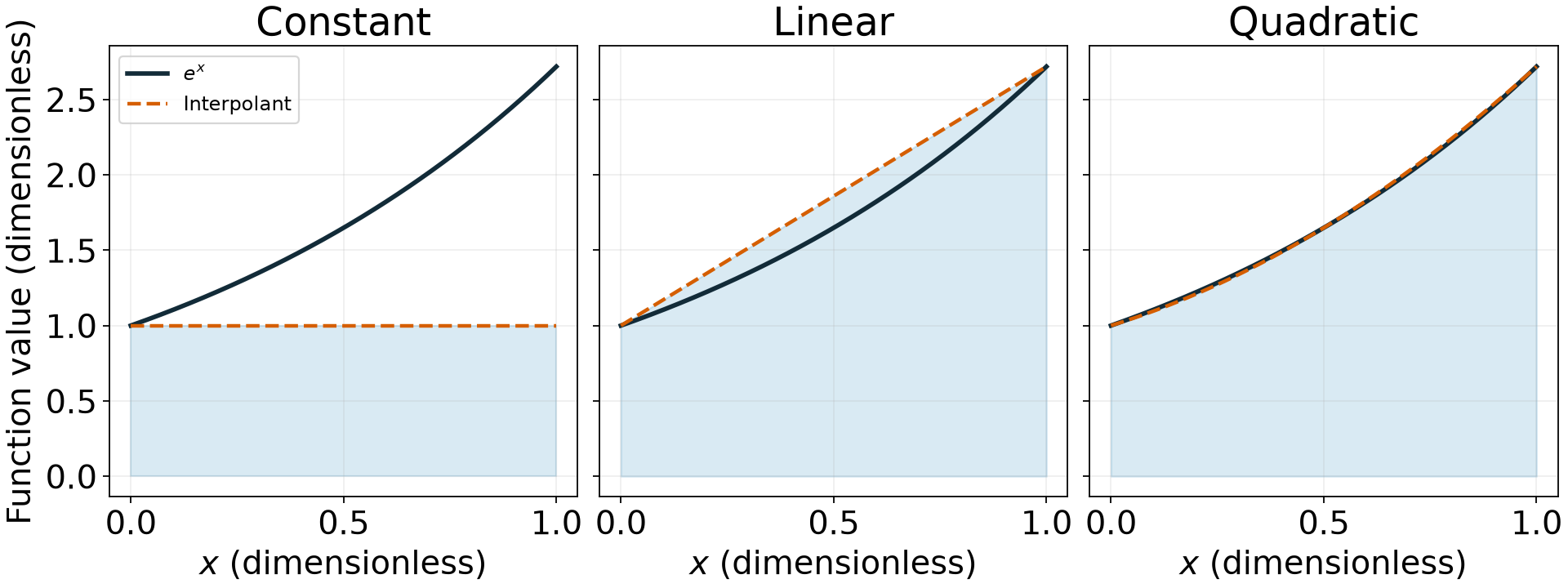
Quadrature integrates the approximating polynomial. The difference between that polynomial and the function determines the quadrature error.
Reference · trapezoid geometry and error
| Feature | Consequence |
|---|---|
| Line through two endpoints | Exact for linear functions in exact arithmetic |
| Interior node shared by two panels | Full interior weight, half endpoint weights |
| Leading local error proportional to h3f′′ | Composite error bounded by a constant times h2 |
| Concave-down integrand | Chords underestimate the area |
Rule: use curvature to predict the error sign before running the calculation.
II · Simpson uses a quadratic and symmetry
Why can an integral gain accuracy beyond the pointwise degree of its interpolant?
Goals
derive weights 1,4,1 across a pair of panels;
explain why composite Simpson requires an even panel count;
use symmetry to explain cubic exactness; and
state the smoothness assumptions behind fourth-order accuracy.
Fit a quadratic across two panels
Let m be the midpoint of a two-panel interval [m−h,m+h]. Write its interpolating quadratic as
The three sample values determine the coefficients:
The integral of Bs over [−h,h] is zero. Therefore
The coefficients give Simpson’s weights
Substitute A and C into the integral:
Here h is the width of one panel. The pair has width 2h.
Check the units and weights: for f(x)=1, the result must be the interval length, 2h. The weights sum to (h/3)(1+4+1)=2h.
Predict: is a cubic integrated exactly? A quadratic interpolant does not reproduce a cubic point by point, so explain your reasoning about its integral.
Symmetry cancels the cubic contribution to the error
Expand a smooth function about the midpoint:
Both the symmetric integral and Simpson’s symmetric weights cancel odd terms. The constant and quadratic contributions agree. The first possible mismatch is the fourth-derivative term.
Derive the Simpson error coefficient
For the fourth-order term, the integral contributes h5fm(4)/60 and Simpson contributes h5fm(4)/36. Their difference is (1/60−1/36)h5fm(4)=−h5fm(4)/90. This identifies the coefficient. The error theorem makes the remainder exact: for f∈C4 on the pair, there is a point ξ in it such that
The paired local error is O(h5) and the composite error is O(h4). For a cubic, the fourth derivative vanishes: Simpson is exact in exact arithmetic.
Pair the panels to build composite Simpson
Endpoint weights: 1.
Odd-index interior weights: 4.
Even-index interior weights: 2 because they join adjacent pairs.
Multiply the sum by h/3.
The panel count n must be positive and even for this composite rule. An odd count is an invalid input, not a reason to silently change the grid.
Translate the weights into array slices
Suppose y = f(nodes) contains the n+1 endpoint heights:
| Expression | Selected values |
|---|---|
y[0], y[-1] | Endpoints |
y[1:-1] | All interior heights, for trapezoid |
y[1:-1:2] | Odd-index interior heights, for Simpson |
y[2:-1:2] | Even-index interior heights, for Simpson |
For n=4, write the five weights on paper. Check that neither endpoint appears inside an interior sum. The complete implementations are your next exercise.
Compare the rectangle samples
Same integrand, same six panels: f(x)=e−x/2cos(2x)+1 on [0,2].
# Plot local interpolants; this is an illustration, not a quadrature library.
from numpy.polynomial import Polynomial
plot_edges = np.linspace(0.0, 2.0, 7)
plot_h = plot_edges[1] - plot_edges[0]
plot_f = lambda x: np.exp(-x/2) * np.cos(2*x) + 1
primitive = lambda x: np.exp(-x/2) * (-0.5*np.cos(2*x) + 2*np.sin(2*x)) / 4.25
plot_exact = 2 + primitive(2) - primitive(0)
for pair, names in enumerate((("Left", "Midpoint"), ("Trapezoid", "Simpson"))):
    fig, axes = plt.subplots(1, 2, figsize=(12, 3.5), layout="constrained")
    for ax, name, color in zip(axes, names, ("#0072B2", "#D55E00")):
        xx = np.linspace(0, 2, 501)
        ax.plot(xx, plot_f(xx), color="#122b38", lw=2)
        area = 0.0
        if pair == 0:
            samples = plot_edges[:-1] + (plot_h/2 if name == "Midpoint" else 0)
            heights = plot_f(samples)
            ax.bar(plot_edges[:-1], heights, width=plot_h, align="edge",
                   color=color, edgecolor=color, alpha=0.25)
            area = plot_h * np.sum(heights)
        else:
            samples = plot_edges
            degree = 1 if name == "Trapezoid" else 2
            for i in range(0, 6, degree):
                nodes = plot_edges[i:i+degree+1]
                poly = Polynomial.fit(nodes, plot_f(nodes), degree)
                xx = np.linspace(nodes[0], nodes[-1], 101)
                ax.fill_between(xx, 0, poly(xx), color=color, alpha=0.25)
                ax.plot(xx, poly(xx), color=color)
                integral = poly.integ()
                area += integral(nodes[-1]) - integral(nodes[0])
        ax.plot(samples, plot_f(samples), "o", color=color)
        ax.set(xlabel="x (dimensionless)", ylabel="f(x)",
               title=f"{name}: {len(samples)} samples\nAbsolute error {abs(area-plot_exact):.3g}")
        ax.tick_params(labelsize=13)
    fig.savefig(f"lecture-06-geometry-{pair}.png", dpi=160)
    plt.close(fig)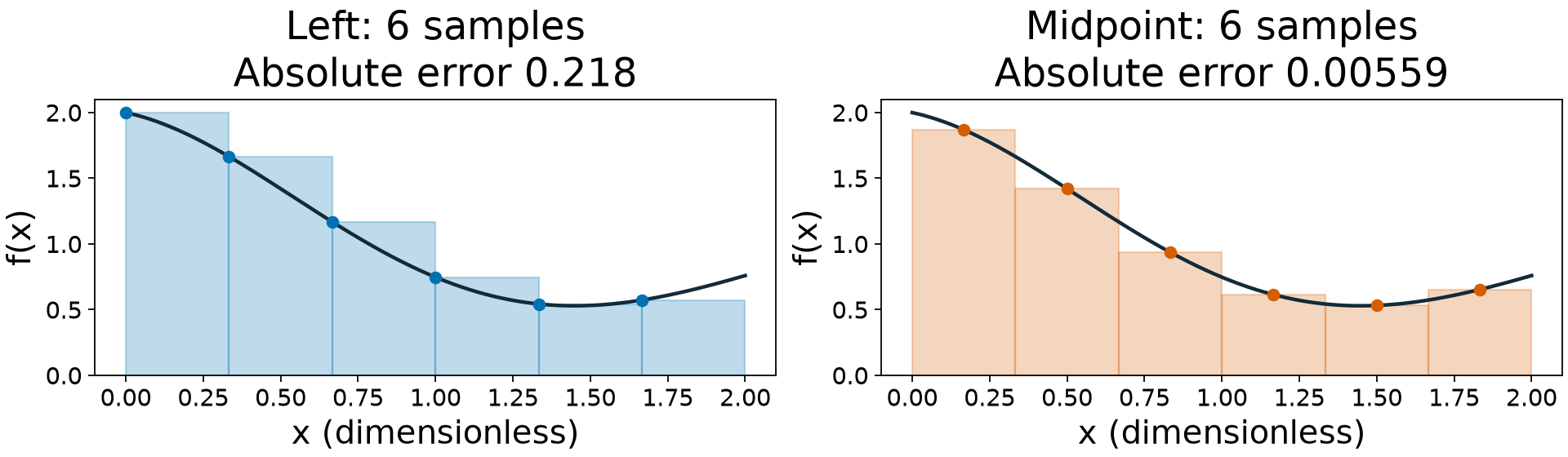
Explain: why does midpoint sampling give the smaller error on this grid?
Compare the endpoint interpolants
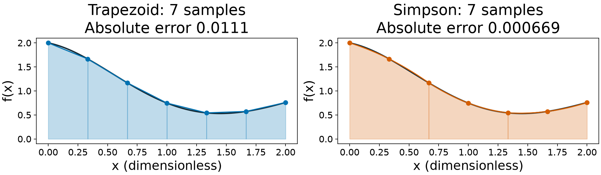
Explain: why do both rules use seven heights for six panels?
Explain the sample count
On this grid, Simpson has the smallest error; midpoint beats trapezoid. One grid does not establish convergence order or a universal ranking.
Explain: why do the endpoint rules need seven sampled heights for six panels? Where do neighboring Simpson pairs reuse a height?
Orders need a smoothness condition
For equal panel widths on a fixed interval:
| Rule | Sufficient derivative bound | Composite error bound |
|---|---|---|
| Left rectangle | M1=max∣f′∣ | (b−a)hM1/2 |
| Trapezoid | M2=max∣f′′∣ | (b−a)h2M2/12 |
| Simpson | M4=max∣f(4)∣ | (b−a)h4M4/180 |
Assume the corresponding derivatives are continuous on [a,b], with a<b. The bounds concern exact-arithmetic quadrature, not floating-point rounding.
When a needed derivative is unbounded or discontinuous, the usual error theorem does not supply that guarantee. We will investigate such an example later.
Reference · a corner changes the error pattern
Interpret: why does the corner in g(x)=ex+∣x−0.2∣ invalidate the usual Simpson bound on [0,1]? Explain the effect of splitting at 0.2.
# Library quadrature produces this illustration; students write their own rules.
from scipy.integrate import simpson as reference_simpson
corner = 0.2
corner_f = lambda x: np.exp(x) + np.abs(x-corner)
corner_exact = np.expm1(1) + (corner**2 + (1-corner)**2)/2
corner_ns = 2**np.arange(2, 11)
corner_errors = [[], [], []]
for panels in corner_ns:
    grid = np.linspace(0, 1, panels+1)
    left = np.linspace(0, corner, panels//2+1)
    right = np.linspace(corner, 1, panels//2+1)
    # Sample the shared endpoint once and reuse its value.
    values = corner_f(np.concatenate((left, right[1:])))
    split_area = (reference_simpson(values[:panels//2+1], x=left)
                  + reference_simpson(values[panels//2:], x=right))
    corner_errors[0].append(abs(reference_simpson(np.exp(grid), x=grid)-np.expm1(1)))
    corner_errors[1].append(abs(reference_simpson(corner_f(grid), x=grid)-corner_exact))
    corner_errors[2].append(abs(split_area-corner_exact))
fig, axes = plt.subplots(1, 2, figsize=(12, 3.7), layout="constrained")
xx = np.linspace(0, 1, 501)
axes[0].plot(xx, corner_f(xx), color="#122b38", lw=2)
axes[0].axvline(corner, color="#D55E00", ls="--")
axes[0].set(xlabel="x", ylabel="g(x)", title="Split at the corner")
for errors, label, color in zip(corner_errors, ("Smooth", "Corner", "Split corner"),
                                ("#0072B2", "#D55E00", "#009E73")):
    axes[1].loglog(corner_ns+1, errors, "o-", label=label, color=color)
axes[1].set(xlabel="Distinct samples", ylabel="Absolute error")
axes[1].legend(fontsize=13)
axes[1].grid(alpha=0.2)
fig.savefig("lecture-06-corner.png", dpi=160)
plt.close(fig)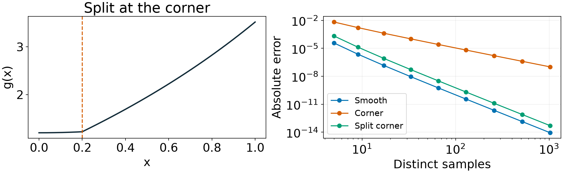
Compare the smooth, unsplit, and split error curves at the same total panel count.
Reference · why splitting at a corner helps
Each calculation uses n+1 distinct samples. The split rule uses half the panels on each side and reuses the shared endpoint.
Each side is smooth: the quadratic no longer crosses the corner. This previews the reading’s investigation. Grid alignment can cancel an error term, so an observed slope alone does not prove smoothness.
Reference · composite Simpson
| Feature | Meaning |
|---|---|
n positive and even | Every panel belongs to a pair |
n + 1 heights | Both boundaries and all interior nodes are sampled |
Weights 1, 4, 2, ..., 4, 1 | Pair weights accumulated across the grid |
Overall factor h / 3 | h is one panel’s width, not a pair’s width |
| Exact cubic integral | A check of weights and indexing, up to rounding |
Rule: polynomial exactness and measured convergence order are different checks.
III · A module gives a function an importable home
How can a notebook and a test call the same numerical implementation?
Goals
separate method definitions from analysis and tests;
import a local module and account for cached notebook imports;
recognize how pytest finds and runs tests; and
translate a stated tolerance into a
pytest.approxassertion.
Give each file one role
quadrature-lab/
├── integrate.py
├── tests/
│   └── test_integrate.py
└── analysis.ipynbintegrate.pydefines numerical methods.The notebook imports them, makes figures, and explains results.
Test files import them and check specified behavior.
A notebook can contain assertions and be tested by execution. Modules make functions easier to import and test independently of notebook state.
Imports connect the files
In a notebook located in the lab directory:
import numpy as np
from integrate import rectangle

estimate = rectangle(np.sin, 0.0, np.pi/2, 100)
Python executes a module’s top-level statements when it first imports it in a process. Keep demonstration runs and plotting out of the module’s top level.
After editing the module, restart the notebook kernel and run from the top. Importing again does not normally reload a module already in memory.
What pytest does
pytest discovers test functions, calls them, and reports failed assertions
and unexpected exceptions.
def test_example():
    result = 2 + 3
    assert result == 5
For this lab, use files named test_*.py and functions named test_*.
An assertion should test a behavior you can explain.
Run from the directory containing integrate.py:
python -m pytestIf pytest is missing, install it in the same course environment with
python -m pip install pytest, then rerun the command.
Carry rtol and atol into tests carefully
NumPy uses rtol and atol. pytest.approx uses rel and abs:
assert actual == pytest.approx(expected, rel=0.0, abs=error_bound)For finite scalar values and both allowances explicitly supplied,
pytest.approx permits a discrepancy up to
NumPy adds its allowances. These APIs therefore differ when both allowances
are nonzero. With rel=0.0, our test has one explicit absolute criterion.
Source: pytest approx documentation.
Reference · modules and tests
| Pattern | Purpose |
|---|---|
from integrate import rectangle | Import the shared implementation |
tests/test_integrate.py | A discoverable home for lab tests |
def test_rectangle_sine(): | One named behavior check |
pytest.approx(reference, rel=0.0, abs=bound) | An explicit absolute comparison |
python -m pytest | Run tests using this Python environment |
Rule: a test should expose a plausible mistake, not repeat the implementation.
IV · Lab: rectangle integration of sine
Can another file import your rule and verify a claim about its result?
Goals
complete an importable rectangle module;
justify a sine-integral test with a derivative bound;
test an invalid-input contract; and
interpret a deliberate failure without weakening a justified criterion.
Predict · the sine integral and the module contract
Work with a partner to discuss the design; write and run your own implementation.
Before typing:
Sketch the curve and two left rectangles.
Predict whether the result is above or below 1.
State which endpoint is omitted from the sampled heights.
Write the input and output contract for
rectangle(f, a, b, n).
Use the known rectangle mathematics to concentrate on modules and tests.
Lab step 1 · Create integrate.py
Start with this skeleton and complete it using Lecture 5:
import numpy as np

def rectangle(f, a, b, n):
    """Approximate an integral using n left rectangles.

    f accepts and returns matching arrays of finite values.
    a and b are finite scalar limits; n is a positive integer.
    Return one float. Invalid n raises ValueError.
    """
    # Validate n, excluding bool and non-integer values.
    # Compute the panel width and n left endpoints.
    # Evaluate f at those endpoints and return the weighted sum.
    raise NotImplementedError("Complete the rectangle rule")
The placeholder is intentional; replace it with your implementation.
Do not hard-code np.sin inside the rule.
Lab step 2 · Choose the tolerance before running the test
Lecture 5 established
For sinx on [0,π/2], M1=max∣cosx∣=1. At n=100, the bound is π2/800≈0.01234.
Use this absolute bound for the known-integral test. The sine result has room below this conservative bound, much larger than rounding effects here.
Explain: a correct left-rectangle rule at n=100 fails a 10-12 accuracy demand here. Why is that a tolerance problem rather than evidence of an implementation bug?
Lab step 3 · Write the known-integral test
Save this in tests/test_integrate.py:
import numpy as np
import pytest
from integrate import rectangle

def test_rectangle_sine():
    n = 100
    estimate = rectangle(np.sin, 0.0, np.pi/2, n)
    error_bound = np.pi**2 / (8*n)
    assert np.isfinite(estimate)
    assert estimate < 1.0  # increasing sine: left rectangles underestimate
    assert estimate == pytest.approx(1.0, rel=0.0, abs=error_bound)
Run python -m pytest. If the test fails, read the actual value and expected
range before changing any code or tolerance.
Lab step 4 · Check invalid inputs
Append this test to the same file:
@pytest.mark.parametrize("bad_n", [0, -2, 2.5, True])
def test_rectangle_rejects_invalid_panel_count(bad_n):
    with pytest.raises(ValueError, match="positive integer"):
        rectangle(np.sin, 0.0, np.pi/2, bad_n)
parametrize runs the function once for each listed value. raises checks the
exception type; match checks the message for the named problem.
If validation is missing, a division error is not the required ValueError.
An error message is part of making the function usable.
Lab step 5 · Make a failure informative
Temporarily change the accuracy tolerance to abs=1e-12, leaving rel=0.0.
Run the test and read the discrepancy it reports.
Is the calculation inconsistent with the first-order bound?
Or is this new accuracy demand unsupported at n=100?
Restore the justified bound, rerun the tests, and import the rule into a clean notebook. Print the estimate and its absolute error.
If time remains, double n and compare the error ratio with the first-order
prediction. The bound test alone does not establish convergence order.
What the lab establishes
| Evidence | Supported claim | Remaining limitation |
|---|---|---|
| Imported function runs | This module is usable from this environment | Other input contracts still need checking |
| Sine test passes | This case meets a justified bound and has the expected sign | One case cannot establish general correctness |
| Invalid counts raise | The listed invalid inputs fail as specified | Other invalid inputs were not tested |
| Error ratio approaches 2 | This sequence is consistent with first-order error | The conclusion is local to the tested regime |
Testing a function, measuring its convergence, and validating a physical model answer different questions.
Documentation for the next question
| Resource | Use it for |
|---|---|
| Python modules tutorial | Imports and module behavior |
| pytest getting started | Test discovery and a first run |
| pytest assertions | Failure reports and expected exceptions |
pytest approx | Absolute and relative comparison semantics |
Read a failure report alongside the test’s stated claim and the function’s contract. Check the documented API before changing the implementation.
Exit check
Why does the trapezoid rule have half weights at the two endpoints?
Why must composite Simpson use an even panel count?
Why can Simpson integrate cubics exactly using quadratic interpolation?
Where do reusable functions, figures, and tests belong?
Why did the lab use
rel=0.0and an absolute error bound?
Carry forward
Implement trapezoid and Simpson with the same callable interface, then measure their convergence. Use a cubic integral as an independent Simpson check.
Your notebook imports the methods and explains their results. Your tests make specific contracts executable. Next class we will use error measurements to assess convergence and choose how much work an accuracy target requires.