Part 2: Statistical Tools and Concepts
How Nature Computes | Statistical Thinking Module 1 | COMP 521
Learning Outcomes
By the end of Part 2, you will be able to:
Distinguish between correlation and independence in physical systems and identify when each assumption is valid
Apply marginalization to reduce complex high-dimensional problems to tractable calculations
Explain ergodicity and why it enables both MCMC sampling and molecular dynamics simulations
Calculate error propagation through multi-step computations using proper statistical rules
Predict when the Law of Large Numbers ensures statistical reliability in astrophysical systems
Apply Bayesian thinking to update beliefs with data using prior knowledge and likelihood
2.1 Correlation and Independence: When Variables Connect
Priority: 🔴 Essential
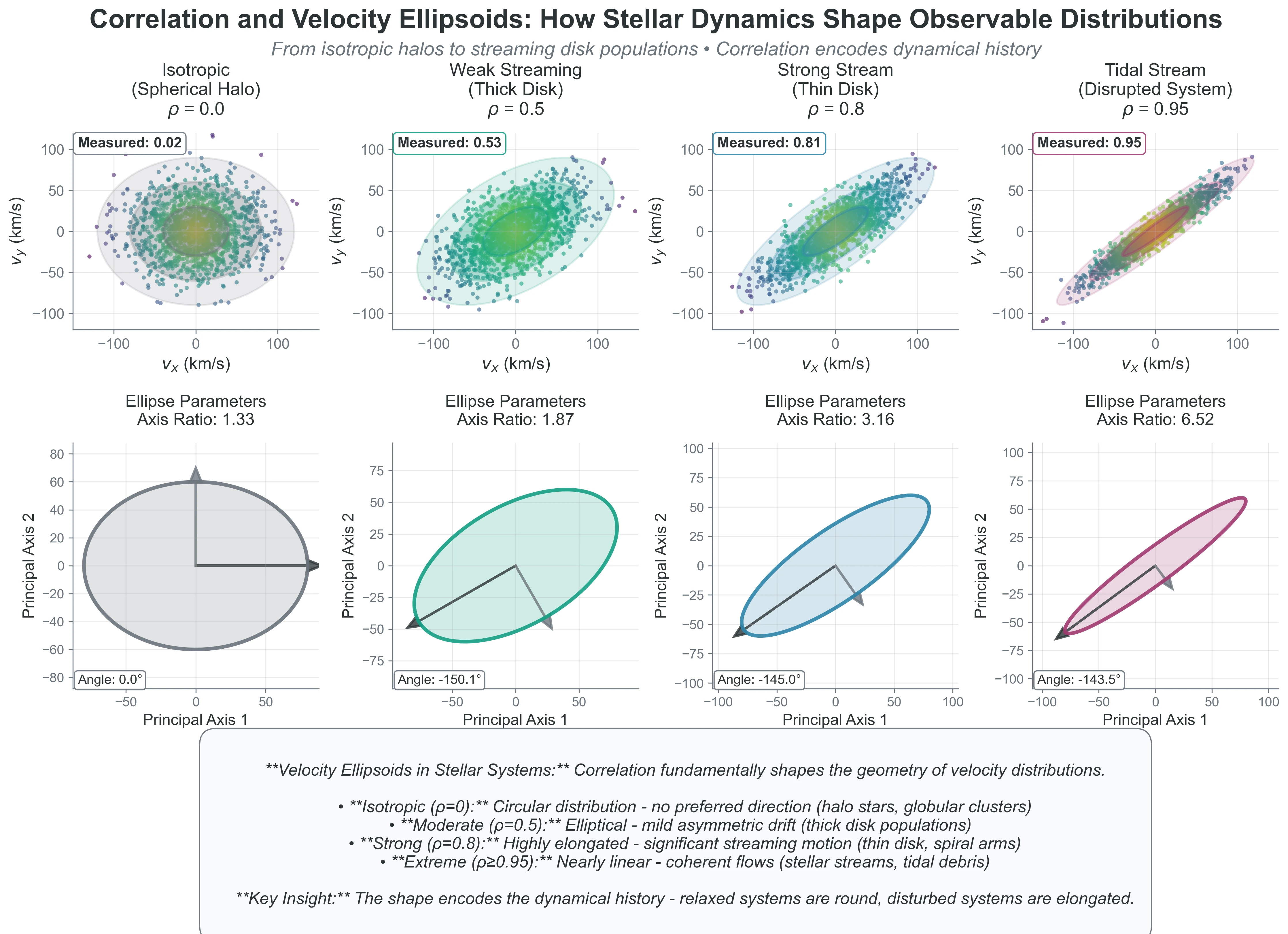
Physical intuition: Watch a flock of starlings move through the sky. When one bird turns, nearby birds turn too. Their velocities aren’t independent — they’re correlated. The same thing happens in stellar streams, where stars that were stripped from the same dwarf galaxy move together through space with correlated velocities.
So far, we’ve assumed particle velocities are independent. But what if they’re not? Understanding correlation is crucial for everything from gas dynamics to Gaussian processes. Correlation feels like structure; precisely, it is dependence encoded in covariance. Catchphrase -> Precision: “Structure in data” means measurable dependence that changes variance, uncertainty, and effective sample size.
💻 Computational Demo: Visualizing Correlation
See how correlation affects the joint distribution of variables:
Code Reliability Contract
Purpose: visualize how covariance structure reshapes joint distributions.
Inputs/Outputs: input is chosen values; output is scatter geometry and measured correlation.
Pitfall: interpreting as independence.
Quick fix: test a nonlinear example (for example and ) and compare covariance versus dependence.
import numpy as np
import matplotlib.pyplot as plt

# Generate correlated velocities with different correlation strengths
fig, axes = plt.subplots(2, 3, figsize=(12, 8))
correlations = [0, 0.3, 0.6, 0.9, -0.5, -0.9]

for idx, rho in enumerate(correlations):
    ax = axes[idx // 3, idx % 3]

    # Generate correlated data using covariance matrix
    mean = [0, 0]
    cov = [[1, rho], [rho, 1]]  # correlation matrix with variance 1
    vx, vy = np.random.multivariate_normal(mean, cov, 1000).T

    # Convert to physical units (km/s for stellar velocities)
    vx = vx * 50  # velocity dispersion ~50 km/s
    vy = vy * 50

    # Plot scatter
    scatter = ax.scatter(vx, vy, alpha=0.5, s=10, c=np.sqrt(vx**2 + vy**2), cmap='viridis')
    ax.set_title(f'rho = {rho}')
    ax.set_xlabel('vx (km/s)')
    ax.set_ylabel('vy (km/s)')
    ax.set_aspect('equal')
    ax.grid(True, alpha=0.3)

    # Add best-fit line to show correlation
    if abs(rho) > 0.3:
        z = np.polyfit(vx, vy, 1)
        p = np.poly1d(z)
        x_line = np.linspace(vx.min(), vx.max(), 100)
        ax.plot(x_line, p(x_line), "r--", alpha=0.5, lw=2)

    # Add text box with statistics
    measured_corr = np.corrcoef(vx, vy)[0,1]
    text_str = f'Measured: {measured_corr:.2f}'
    ax.text(0.05, 0.95, text_str, transform=ax.transAxes,
            verticalalignment='top', bbox=dict(boxstyle='round', facecolor='wheat', alpha=0.5))

plt.suptitle('How Correlation Shapes Velocity Distributions', fontsize=14)
plt.tight_layout()
plt.show()

# Show how correlation affects the velocity ellipsoid
print("Effect of correlation on velocity ellipsoid:")
print("-" * 50)
for rho in [0, 0.5, 0.9]:
    cov = [[1, rho], [rho, 1]]
    eigenvalues, eigenvectors = np.linalg.eig(cov)
    print(f"rho = {rho}:")
    print(f"  Principal axes ratios: {eigenvalues[0]:.2f} : {eigenvalues[1]:.2f}")
    print(f"  Ellipse rotation angle: {np.degrees(np.arctan2(eigenvectors[1,0], eigenvectors[0,0])):.1f} degrees")
Key insights:
: Circular distribution (isotropic velocities)
: Elliptical, tilted toward positive correlation
: Elliptical, tilted toward negative correlation
: Distribution collapses toward a line
Copy/paste quick-check: Imports: numpy, matplotlib. Seed recommendation: set np.random.seed(536) for reproducible scatter realizations. Variability: measured sample correlations fluctuate around target values.
Physical examples of correlation:
Ideal gas: Particle velocities are independent
Pressure tensor is diagonal:
No shear stress, no viscosity
Stellar streams: Velocities are correlated
Stars moving together have correlated velocities
Off-diagonal pressure terms represent streaming motion
Turbulence: Strong velocity correlations
Eddies create correlated motion
Kolmogorov spectrum from correlation functions
Why correlation matters for your projects:
Project 2 (N-body): Initially uncorrelated velocities become correlated through gravity
Stars in the same cluster develop correlated orbits
Tidal streams show strong velocity correlations
Project 4 (MCMC): Autocorrelation determines effective sample size
High correlation = slow exploration
Need to account for correlation in error estimates
Effective sample size: where is integrated autocorrelation time (convention-dependent; equivalent forms like are also used)
Project 5 (Gaussian Processes): Entire method based on correlation!
Covariance kernel defines correlation between points
Predictions use correlations to interpolate
Project Hook: This appears in Project 4 when you convert autocorrelation into an effective sample size before trusting posterior uncertainty.
 {#fig-correlation-velocity-ellipsoids width=“100%”}
The key insight: Independence makes problems tractable (can multiply probabilities). Correlation makes problems realistic (real systems have relationships). Understanding when to assume independence and when to model correlation is crucial for both physics and ML.
2.2 Marginalization: The Art of Ignoring
Priority: 🔴 Essential
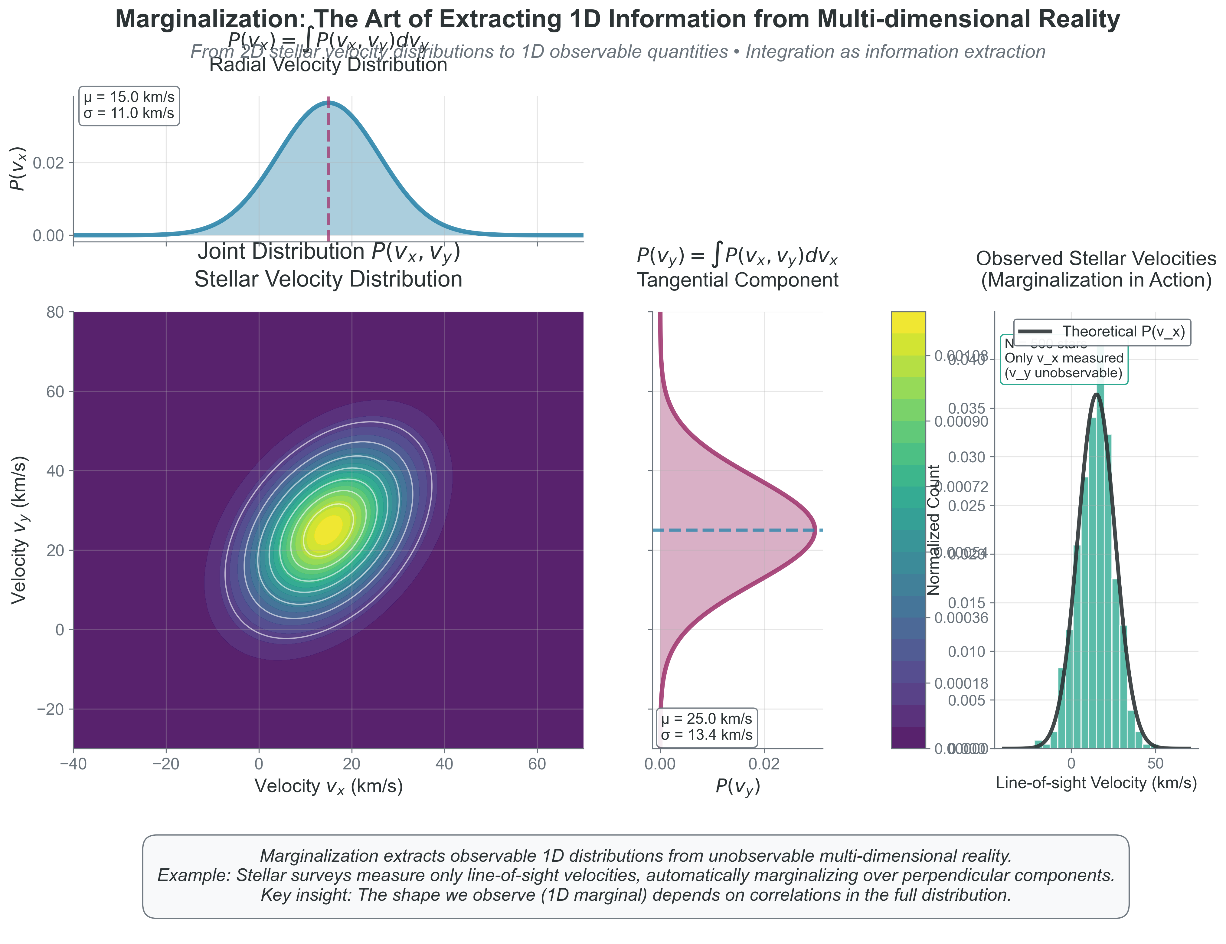
Physical intuition: Imagine a 3D sculpture casting a shadow on a wall. The 2D shadow is a marginalization of the 3D object — you’ve integrated out the depth dimension. Similarly, when we observe stellar velocities along the line of sight, we’re seeing a marginalization of the full 3D velocity distribution.
We have velocities in 3D but often need just speeds. We know positions and velocities but only care about energy. How do we extract what matters? Through marginalization — integrating out unwanted variables.
The mathematical operation:
“Sum over all possible values of what you don’t care about.”
These demos use numpy, matplotlib, and scipy; if SciPy is missing, run pip install scipy.
💻 Computational Demo: Marginalization in Action
Watch how we go from 2D joint distributions to 1D marginal distributions:
import numpy as np
import matplotlib.pyplot as plt
from scipy import stats

# Create a 2D joint distribution (correlated Gaussian)
mean = [2, 3]
cov = [[1, 0.7], [0.7, 2]]
rv = stats.multivariate_normal(mean, cov)

# Create grid for visualization
x = np.linspace(-2, 6, 100)
y = np.linspace(-2, 8, 100)
X, Y = np.meshgrid(x, y)
pos = np.dstack((X, Y))
Z = rv.pdf(pos)

# Setup figure
fig = plt.figure(figsize=(12, 8))
gs = fig.add_gridspec(3, 3, width_ratios=[2, 1, 0.5], height_ratios=[1, 2, 0.5])

# Main 2D distribution
ax_joint = fig.add_subplot(gs[1, 0])
contour = ax_joint.contourf(X, Y, Z, levels=20, cmap='viridis')
ax_joint.set_xlabel('X (e.g., velocity_x)')
ax_joint.set_ylabel('Y (e.g., velocity_y)')
ax_joint.set_title('Joint Distribution P(X,Y)')

# Marginal distribution for X (top)
ax_margx = fig.add_subplot(gs[0, 0], sharex=ax_joint)
marginal_x = np.trapz(Z, y, axis=0)  # Integrate over y
marginal_x = marginal_x / np.trapz(marginal_x, x)  # Normalize
ax_margx.plot(x, marginal_x, 'b-', lw=2)
ax_margx.fill_between(x, marginal_x, alpha=0.3)
ax_margx.set_ylabel('P(X)')
ax_margx.set_title('Marginal P(X) = ∫P(X,Y)dY')
plt.setp(ax_margx.get_xticklabels(), visible=False)

# Marginal distribution for Y (right)
ax_margy = fig.add_subplot(gs[1, 1], sharey=ax_joint)
marginal_y = np.trapz(Z, x, axis=1)  # Integrate over x
marginal_y = marginal_y / np.trapz(marginal_y, y)  # Normalize
ax_margy.plot(marginal_y, y, 'r-', lw=2)
ax_margy.fill_betweenx(y, marginal_y, alpha=0.3)
ax_margy.set_xlabel('P(Y)')
ax_margy.set_title('P(Y) = ∫P(X,Y)dX')
plt.setp(ax_margy.get_yticklabels(), visible=False)

# Add colorbar
ax_cb = fig.add_subplot(gs[1, 2])
plt.colorbar(contour, cax=ax_cb, label='Probability Density')

# Add text explanation
ax_text = fig.add_subplot(gs[2, :])
ax_text.axis('off')
ax_text.text(0.5, 0.5,
             'Marginalization: To get P(X), integrate out Y. To get P(Y), integrate out X.\n' +
             'Physical example: Observing only radial velocity (1D) from 3D velocity distribution.',
             ha='center', va='center', fontsize=12, bbox=dict(boxstyle='round', facecolor='wheat'))

plt.suptitle('Marginalization: From Joint to Marginal Distributions', fontsize=14)
plt.tight_layout()
plt.show()

# Quantitative analysis
print("Statistics of the distributions:")
print("-" * 50)
print(f"Joint distribution mode: X={mean[0]:.1f}, Y={mean[1]:.1f}")
print(f"Marginal X: mean={np.trapz(x*marginal_x, x):.2f}, std={np.sqrt(np.trapz((x-mean[0])**2*marginal_x, x)):.2f}")
print(f"Marginal Y: mean={np.trapz(y*marginal_y, y):.2f}, std={np.sqrt(np.trapz((y-mean[1])**2*marginal_y, y)):.2f}")
Copy/paste quick-check: Imports: numpy, matplotlib, scipy. Seed recommendation: set np.random.seed(536) before sampling for reproducible contour examples. Variability: exact contour noise and moment estimates vary slightly across runs.
Example: From 3D velocities to 1D speeds
Starting with Maxwell-Boltzmann in 3D:
To get speed distribution, integrate over all directions:
📝 Step-by-Step: Where the factor comes from
To marginalize from velocity vectors to speeds, we integrate over all directions:
Convert to spherical coordinates:
The Jacobian:
Integrate over angles:
Since only depends on (isotropic):
The factor has a geometric meaning: It’s the surface area of a spherical shell in velocity space. There are more ways to have large speeds than small speeds — more directions point to the same speed magnitude!
This is why the Maxwell speed distribution peaks at non-zero velocity even though the velocity distribution (for each component) peaks at zero.
Marginalization appears everywhere:
| Context | Marginalizing Over | To Get |
|---|---|---|
| Bayesian inference | Nuisance parameters | Posterior of interest |
| Gaussian Processes | Unobserved points | Predictions at test points |
| Statistical mechanics | Microscopic details | Macroscopic observables |
| Neural networks | Hidden layers | Output predictions |
| Image processing | Noise dimensions | Clean signal |
The profound pattern: Complex high-dimensional problem Marginalize Simple low-dimensional answer
This is how we go from 1057 particle coordinates to 4 stellar structure equations!
 {#fig-marginalization-visualization width=“100%”}
What to notice:
The 1D radial-velocity histogram is a marginal of a higher-dimensional distribution.
Correlation in the joint distribution changes the shape and width of each marginal.
Observations rarely give the full state; inference depends on careful marginalization.
2.3 Ergodicity: When Time Equals Ensemble
Priority: 🔴 Essential
Physical intuition: Drop a blob of cream into your coffee. At first, it stays localized. But as you stir (or just wait), the cream explores the entire cup. Eventually, any small region has the same cream concentration as the time-average. This is ergodicity — one particle’s journey through time tells you about all possible states.
You measure the pressure of a gas over time. You also calculate the ensemble average over all possible microstates. Remarkably, these give the same answer. This is ergodicity — one of the deepest principles in statistical mechanics.
Assumption break cue: This relation can fail in finite windows when stationarity is not reached or when trajectories remain trapped in weakly connected regions.
In finite simulations, we compare time averages to expectations under a stationary distribution and still check stationarity and mixing before trusting the match.
💻 Computational Demo: Ergodic vs Non-Ergodic Systems
See the difference between ergodic and non-ergodic behavior:
import numpy as np
import matplotlib.pyplot as plt

# Simulate two systems: mixing stochastic vs quasi-periodic
fig, axes = plt.subplots(2, 3, figsize=(14, 8))
t = np.linspace(0, 100, 10000)
dt = t[1] - t[0]
rng = np.random.default_rng(42)

# System 1: Mixing stochastic dynamics (ergodic w.r.t. stationary distribution)
x_ergodic = np.zeros_like(t)
v_ergodic = np.zeros_like(t)
for i in range(1, len(t)):
    # Damped stochastic oscillator (Langevin-like)
    v_ergodic[i] = 0.97 * v_ergodic[i-1] - 0.15 * x_ergodic[i-1] + 0.25 * rng.normal()
    x_ergodic[i] = x_ergodic[i-1] + v_ergodic[i] * dt

# System 2: Quasi-periodic torus orbit (non-ergodic on full phase space)
x_nonergodic = np.sin(t) + 0.25*np.sin(np.sqrt(2)*t)
v_nonergodic = np.cos(t) + 0.25*np.cos(np.sqrt(2)*t)

# Plot trajectories in phase space
axes[0, 0].plot(x_ergodic[:1000], v_ergodic[:1000], 'b-', alpha=0.5, lw=0.5)
axes[0, 0].set_title('Mixing stochastic: Early time (t<10)')
axes[0, 0].set_xlabel('Position')
axes[0, 0].set_ylabel('Velocity')

axes[0, 1].plot(x_ergodic[:5000], v_ergodic[:5000], 'b-', alpha=0.3, lw=0.5)
axes[0, 1].set_title('Mixing stochastic: Medium time (t<50)')
axes[0, 1].set_xlabel('Position')

axes[0, 2].plot(x_ergodic, v_ergodic, 'b-', alpha=0.2, lw=0.5)
axes[0, 2].set_title('Mixing stochastic: Long time\nExplores stationary region')
axes[0, 2].set_xlabel('Position')

# Non-ergodic
axes[1, 0].plot(x_nonergodic[:1000], v_nonergodic[:1000], 'r-', alpha=0.5, lw=0.5)
axes[1, 0].set_title('Quasi-periodic: Early time')
axes[1, 0].set_xlabel('Position')
axes[1, 0].set_ylabel('Velocity')

axes[1, 1].plot(x_nonergodic[:5000], v_nonergodic[:5000], 'r-', alpha=0.5, lw=0.5)
axes[1, 1].set_title('Quasi-periodic: Medium time')
axes[1, 1].set_xlabel('Position')

axes[1, 2].plot(x_nonergodic, v_nonergodic, 'r-', alpha=0.5, lw=0.5)
axes[1, 2].set_title('Quasi-periodic: Long time\nConfined to invariant curve')
axes[1, 2].set_xlabel('Position')

# Set consistent axes
for ax in axes.flat:
    ax.set_xlim(-2, 2)
    ax.set_ylim(-2, 2)
    ax.grid(True, alpha=0.3)
    ax.set_aspect('equal')

plt.suptitle('Ergodic vs Non-Ergodic Systems in Phase Space', fontsize=14)
plt.tight_layout()
plt.show()

# Demonstrate time average vs stationary-distribution proxy for mixing system
print("Checking ergodicity: Time average vs stationary-distribution proxy")
print("-" * 50)

# Time average of x^2
time_avg = np.mean(x_ergodic**2)

# Stationary-distribution proxy from independent draws near stationarity
proxy_values = []
for i in range(1000):
    x_sample = rng.normal(loc=0.0, scale=np.std(x_ergodic))
    proxy_values.append(x_sample**2)
proxy_avg = np.mean(proxy_values)

print("Mixing stochastic system:")
print(f"  Time average of x^2: {time_avg:.3f}")
print(f"  Stationary-distribution proxy for x^2: {proxy_avg:.3f}")
print(f"  Difference: {abs(time_avg - proxy_avg):.4f} ← Should be small!")

# For non-ergodic, they differ
time_avg_non = np.mean(x_nonergodic**2)
print(f"\nNon-ergodic system:")
print(f"  Time average of x^2: {time_avg_non:.3f}")
print(f"  Would need multiple trajectories for a trustworthy stationary expectation estimate")
Copy/paste quick-check: Imports: numpy, matplotlib. Seed: built in (np.random.default_rng(42)) for reproducibility. Variability: deterministic for fixed seed; changing seed alters stochastic-trajectory details.
Why ergodicity matters:
For physics: We can’t measure ensemble averages directly (need all possible microstates). But we can measure time averages! Ergodicity says they’re the same.
For MCMC (Project 4): Your Markov chain explores parameter space over “time” (iterations). Under stationarity and adequate mixing:
Chain averages can approximate posterior expectations
One long well-mixed chain can emulate many independent samples up to
Burn-in removes clear pre-stationary transients, but diagnostics are still required
For molecular dynamics: Simulate one system over time instead of many systems at once
When ergodicity fails:
Glasses: Stuck in local configuration (non-ergodic)
Broken symmetry: System can’t access all states
Isolated systems: No mixing between regions
The profound connection: Ergodicity links:
Theoretical (ensemble averages)
Computational (time evolution)
Experimental (time measurements)
All give the same answer for ergodic systems!
When Can We Assume Ergodicity?
Key diagnostic questions:
Mixing time vs. observation time: Is ?
Phase space connectivity: Can the system reach all allowed states?
Energy barriers: Are there insurmountable barriers between regions?
Practical examples:
Gas molecules: , seconds effectively ergodic
Protein folding: milliseconds, but can get stuck in local minima can be non-ergodic on finite windows
MCMC chains: require irreducibility/aperiodicity and sufficient mixing length for reliable ergodic averages
The MCMC connection (crucial for Project 4): Your Markov chain starts out of stationarity (often near an arbitrary initial guess). After burn-in, we diagnose convergence and mixing before treating chain averages as posterior expectations. The integrated autocorrelation time sets the effective sample size. This is why we:
Discard burn-in samples (pre-stationary transients)
Estimate effective sample size from (thinning optional and context-dependent)
Run multiple chains and check diagnostics (for example and ESS)
2.4 The Law of Large Numbers: Why Statistics Works
Priority: 🔴 Essential
All these statistical principles work because of a mathematical miracle: as , randomness vanishes.
The Law of Large Numbers (LLN): For independent samples with standard deviation , the standard error of the sample mean scales as:
Typical relative fluctuations of an average therefore scale as (while the variance of the mean scales as ).
Assumption break cue: This scaling can fail when samples are strongly correlated, variance is infinite, or effective sample size is much smaller than nominal .
💻 Computational Demo: Watching Fluctuations Vanish
See how increasing N makes averages more stable:
import numpy as np
import matplotlib.pyplot as plt
# Demonstrate convergence with increasing N
fig, axes = plt.subplots(2, 2, figsize=(12, 8))
# Different N values to test
N_values = [10, 100, 1000, 10000, 100000]
colors = ['red', 'orange', 'yellow', 'green', 'blue']
# Top left: Show sample averages for different N
ax = axes[0, 0]
for N, color in zip(N_values, colors):
# Generate many realizations
n_realizations = 1000
averages = []
for _ in range(n_realizations):
sample = np.random.normal(0, 1, N)
averages.append(np.mean(sample))
# Plot distribution of averages
bins = np.linspace(-1, 1, 50)
ax.hist(averages, bins=bins, alpha=0.5, label=f'N={N}', color=color, density=True)
ax.set_xlabel('Sample Average')
ax.set_ylabel('Probability Density')
ax.set_title('Distribution of Averages Narrows with N')
ax.legend()
ax.set_xlim(-1, 1)
# Top right: Log-log plot of standard deviation vs N
ax = axes[0, 1]
N_range = np.logspace(1, 6, 50, dtype=int)
std_devs = []
for N in N_range:
# Calculate standard deviation of the mean
n_trials = 100
means = [np.mean(np.random.normal(0, 1, N)) for _ in range(n_trials)]
std_devs.append(np.std(means))
ax.loglog(N_range, std_devs, 'bo-', alpha=0.5, label='Measured')
ax.loglog(N_range, 1/np.sqrt(N_range), 'r--', lw=2, label=r'$1/\sqrt{N}$ theory')
ax.set_xlabel('Number of Samples (N)')
ax.set_ylabel('Standard Deviation of Mean')
ax.set_title(r'Universal $1/\sqrt{N}$ Scaling')
ax.legend()
ax.grid(True, alpha=0.3)
# Bottom left: Convergence visualization
ax = axes[1, 0]
N_max = 10000
running_avg = np.cumsum(np.random.normal(0, 1, N_max)) / np.arange(1, N_max+1)
running_std = 1/np.sqrt(np.arange(1, N_max+1))
ax.plot(running_avg, 'b-', alpha=0.7, label='Running average')
ax.fill_between(range(N_max), running_std, -running_std, alpha=0.3, color='red', label='+/- 1 sigma bounds')
ax.set_xlabel('Number of Samples')
ax.set_ylabel('Running Average')
ax.set_title('Convergence to True Mean (0)')
ax.set_xlim(0, N_max)
ax.legend()
# Bottom right: Physical scales
ax = axes[1, 1]
scales = ['Small box\n(N~100)', 'Room\n(N~10^26)', 'Star\n(N~10^57)', 'Galaxy\n(N~10^68)']
N_phys = [100, 1e26, 1e57, 1e68]
fluctuations = [1/np.sqrt(N) for N in N_phys]
bars = ax.bar(scales, fluctuations, color=['red', 'orange', 'green', 'blue'])
ax.set_ylabel('Relative Fluctuation')
ax.set_yscale('log')
ax.set_title('Why Macroscopic Physics is Stable')
ax.set_ylim(1e-35, 1)
# Add annotations
for bar, fluct in zip(bars, fluctuations):
height = bar.get_height()
ax.text(bar.get_x() + bar.get_width()/2., height*2,
f'{fluct:.1e}', ha='center', va='bottom')
plt.suptitle('The Law of Large Numbers: How N Conquers Randomness', fontsize=14)
plt.tight_layout()
plt.show()
# Quantitative analysis
print("Fluctuation scaling with N:")
print("-" * 50)
for N in [100, 1e6, 1e23, 1e57]:
fluct = 1/np.sqrt(N)
print(f"N = {N:.0e}: Fluctuations ~ {fluct:.2e} ({fluct*100:.2e}%)")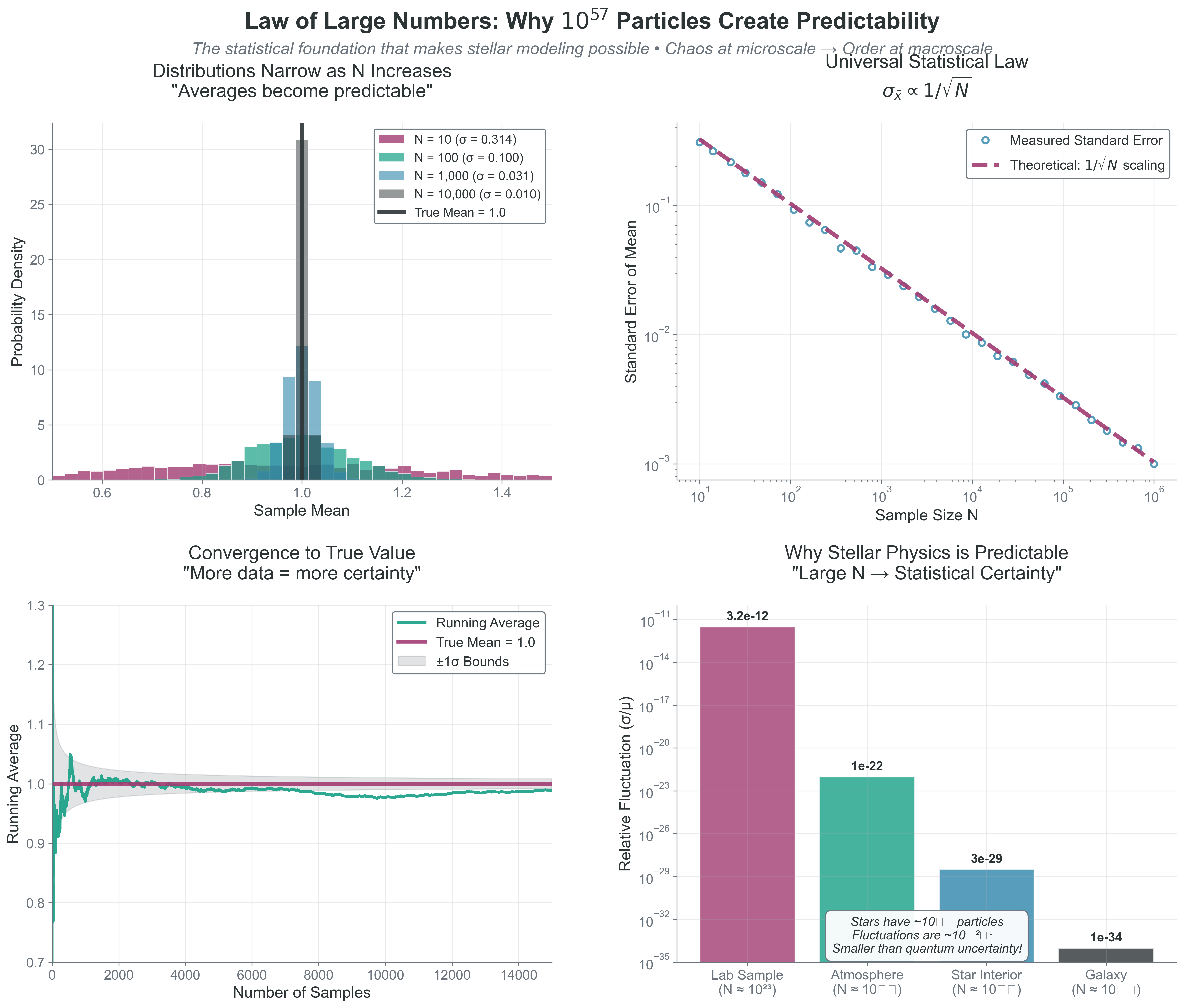 {#fig-law-of-large-numbers-convergence width=“100%”}
Copy/paste quick-check: Imports: numpy, matplotlib. Seed recommendation: set np.random.seed(536) before drawing samples if you want repeatable histograms. Variability: slope and narrowing trend should hold, but individual trajectories/histograms vary.
What this means:
: ~10% fluctuations
: ~0.1% fluctuations
: ~10-11% fluctuations
(Sun): ~10-28% fluctuations
At stellar scales, fluctuations are smaller than quantum uncertainty!
This is why:
Pressure is steady despite chaotic collisions
Stars shine steadily despite random fusion events
Thermodynamics works despite molecular chaos
Monte Carlo methods converge despite using random numbers
This scaling has profound implications for how errors propagate through calculations, which we’ll explore next.
2.5 Error Propagation: The Universal Scaling
Priority: 🟡 Standard Path
Every measurement has uncertainty. Every calculation propagates these uncertainties. Understanding error propagation is crucial for both physics and computation. The Law of Large Numbers tells us fluctuations scale as — now let’s see how this propagates through calculations.
Assumption break cue: First-order propagation can fail for strongly nonlinear mappings, non-Gaussian uncertainties, or omitted covariance structure.
💻 Computational Demo: Error Propagation in Action
See how errors propagate through calculations:
import numpy as np
import matplotlib.pyplot as plt

# Example: Calculate stellar luminosity from radius and temperature
# Use proportional form only: L ~ R**2 * T**4

# "Measurements" with uncertainties
R_mean = 1.0  # Solar radii
R_sigma = 0.05  # 5% uncertainty
T_rel_mean = 1.0  # T / T_sun
T_rel_sigma = 50 / 5778  # fractional temperature uncertainty

# Method 1: Error propagation formula
# L = R^2 * T_rel^4, so:
# dL/dR = 2*R*T_rel^4
# dL/dT_rel = 4*R^2*T_rel^3
L_mean = R_mean**2 * T_rel_mean**4

dL_dR = 2 * R_mean * T_rel_mean**4
dL_dT = 4 * R_mean**2 * T_rel_mean**3

L_sigma_formula = np.sqrt((dL_dR * R_sigma)**2 + (dL_dT * T_rel_sigma)**2)
L_relative_error_formula = L_sigma_formula / L_mean

# Method 2: Monte Carlo error propagation
n_samples = 10000
R_samples = np.random.normal(R_mean, R_sigma, n_samples)
T_rel_samples = np.random.normal(T_rel_mean, T_rel_sigma, n_samples)
L_samples = R_samples**2 * T_rel_samples**4

L_mean_MC = np.mean(L_samples)
L_sigma_MC = np.std(L_samples)
L_relative_error_MC = L_sigma_MC / L_mean_MC

# Visualization
fig, axes = plt.subplots(2, 2, figsize=(12, 10))

# Top left: Input distributions
ax = axes[0, 0]
ax.hist(R_samples/R_mean, bins=50, alpha=0.5, density=True, label='R/R_sun')
ax.hist(T_rel_samples/T_rel_mean, bins=50, alpha=0.5, density=True, label='T/T_sun')
ax.set_xlabel('Normalized Value')
ax.set_ylabel('Probability Density')
ax.set_title('Input Distributions')
ax.legend()

# Top right: Output distribution
ax = axes[0, 1]
ax.hist(L_samples/L_mean, bins=50, density=True, alpha=0.7, color='green')
ax.axvline(1, color='red', linestyle='--', label='True value')
ax.set_xlabel('L / L_ref')
ax.set_ylabel('Probability Density')
ax.set_title(f'Luminosity Distribution\nsigma_L/L = {L_relative_error_MC:.1%}')
ax.legend()

# Bottom left: Error contributions
ax = axes[1, 0]
# Calculate individual contributions
L_from_R_only = R_samples**2 * T_rel_mean**4
L_from_T_only = R_mean**2 * T_rel_samples**4
R_contribution = np.std(L_from_R_only) / L_mean
T_contribution = np.std(L_from_T_only) / L_mean

contributions = [R_contribution*100, T_contribution*100, L_relative_error_MC*100]
labels = ['R uncertainty\nalone', 'T uncertainty\nalone', 'Total\n(combined)']
colors = ['blue', 'red', 'green']

bars = ax.bar(labels, contributions, color=colors, alpha=0.7)
ax.set_ylabel('Relative Error (%)')
ax.set_title('Error Contributions')

# Add values on bars
for bar, val in zip(bars, contributions):
    ax.text(bar.get_x() + bar.get_width()/2, bar.get_height()*1.05,
            f'{val:.1f}%', ha='center', fontsize=10)

# Bottom right: Comparison of methods
ax = axes[1, 1]
ax.text(0.1, 0.8, 'Error Propagation Comparison:', fontsize=12, weight='bold')
ax.text(0.1, 0.6, f'Formula method: sigma_L/L = {L_relative_error_formula:.2%}', fontsize=11)
ax.text(0.1, 0.5, f'Monte Carlo method: sigma_L/L = {L_relative_error_MC:.2%}', fontsize=11)
ax.text(0.1, 0.3, 'Key insight:', fontsize=11, style='italic')
ax.text(0.1, 0.2, 'T^4 dependence means T errors dominate!', fontsize=11)
ax.text(0.1, 0.1, f'(T contrib: {T_contribution/L_relative_error_MC:.1%} of total)', fontsize=10)
ax.axis('off')

plt.suptitle('Error Propagation: From Input Uncertainties to Output', fontsize=14)
plt.tight_layout()
plt.show()

print("Error Propagation Analysis:")
print("-" * 50)
print(f"Input uncertainties:")
print(f"  R: {R_sigma/R_mean:.1%}")
print(f"  T/T_sun: {T_rel_sigma/T_rel_mean:.1%}")
print(f"\nOutput uncertainty in L:")
print(f"  Formula method: {L_relative_error_formula:.2%}")
print(f"  Monte Carlo: {L_relative_error_MC:.2%}")
print(f"\nError contributions:")
print(f"  From R uncertainty: {R_contribution:.2%}")
print(f"  From T uncertainty: {T_contribution:.2%}")
print(f"  Ratio T/R contribution: {T_contribution/R_contribution:.1f}x")
Key insights from this example:
dependence means temperature errors dominate luminosity uncertainty
Formula and Monte Carlo methods agree (validating both)
Understanding error propagation helps identify which measurements need improvement
Copy/paste quick-check: Imports: numpy, matplotlib. Seed recommendation: set np.random.seed(536) before sampling to reproduce relative-error outputs. Variability: exact percentage values vary, but sensitivity should remain dominant.
Monte Carlo error scaling:
For samples, the error in the mean scales as:
This scaling is universal:
Want 10 better accuracy? Need 100 more samples
Diminishing returns as increases
Why Monte Carlo can be slow but always converges
Application to your projects:
Project 2: Energy-error behavior depends on integrator choice: symplectic schemes typically show bounded oscillatory , while non-symplectic schemes can drift over long runs. Diagnose this empirically with a vs time plot and timestep refinement tests.
Project 3: Monte Carlo photon error decreases as
Project 4: MCMC error includes autocorrelation:
Here is the integrated autocorrelation time (convention-dependent; equivalent forms are common).
2.6 Variance and Standard Deviation: Measuring Spread
Priority: 🔴 Essential
While the mean tells us where a distribution is centered, variance and standard deviation tell us how spread out it is — crucial for understanding everything from temperature to measurement uncertainty.
Definitions: Variance: The average squared deviation from the mean
Standard Deviation: The square root of variance
Why square root? It puts the measure back in the same units as the original data.
Physical Interpretation
Remember from Part 1: Temperature IS proportional to velocity variance
This isn’t an analogy — it’s an identity. Higher temperature literally means larger variance in molecular velocities.
Key Properties
Variance of a sum (independent variables):
Variance of a scaled variable:
Standard error of the mean:
This is why averaging reduces uncertainty!
Why This Matters for Your Projects
Project 2: Velocity dispersion in star clusters is literally the standard deviation of stellar velocities
Project 3: Photon count uncertainty follows Poisson statistics where variance equals the mean
Project 4: MCMC convergence diagnosed by monitoring variance between chains
Project 5: Gaussian Process variance gives uncertainty bands on predictions
The takeaway: Variance isn’t just a statistical concept — it’s often the physical quantity we’re measuring (temperature, pressure, velocity dispersion).
2.7 Bayesian Thinking: Learning from Data
Priority: 🔴 Essential Physical intuition: You observe a star with a reddish color. Is it red because it’s an intrinsically cool M-dwarf, or is it a hotter star reddened by interstellar dust? Your prior knowledge (most nearby stars aren’t heavily reddened) combines with the observation (the color) to give you a posterior belief about the star’s true nature. This is Bayesian inference — using prior knowledge plus new data to update beliefs.
Bayes’ Theorem: The Learning Equation
At its heart, Bayesian inference is about updating beliefs with data:
Or in the notation you’ll use constantly:
where:
Prior : What you believed about parameters before seeing data
Likelihood : How probable the data is if parameters are
Posterior : Updated belief after incorporating data
Evidence : Normalization ensuring probabilities sum to 1
💻 Computational Demo: Bayesian Learning in Action
See how prior beliefs update with data to give posterior knowledge:
import numpy as np
import matplotlib.pyplot as plt
from scipy import stats

# Example: Inferring a star's temperature from its color
# Color index B-V is related to temperature, but with uncertainty

fig, axes = plt.subplots(2, 3, figsize=(14, 8))

# True stellar temperature (unknown to us)
T_true = 5800  # K (Sun-like)

# Prior: Based on stellar population studies
# Most stars are cool (M-dwarfs), fewer hot stars
T_range = np.linspace(3000, 10000, 1000)

# Prior: Log-normal distribution (more cool stars)
prior_mean = np.log(4500)
prior_std = 0.4
prior = stats.lognorm.pdf(T_range, s=prior_std, scale=np.exp(prior_mean))
prior = prior / np.trapz(prior, T_range)  # Normalize

# Observation: Color measurement with uncertainty
# Simplified relation: B-V ~ 5000/T (very approximate!)
observed_color = 5000/T_true + np.random.normal(0, 0.1)
color_uncertainty = 0.1

# Likelihood: probability of data given temperature
def likelihood(T, observed_color, uncertainty):
    expected_color = 5000/T  # Our model
    return stats.norm.pdf(observed_color, expected_color, uncertainty)

like = np.array([likelihood(T, observed_color, color_uncertainty) for T in T_range])
like = like / np.trapz(like, T_range)  # Normalize for visualization

# Posterior: Prior $\times$ Likelihood (then normalize)
posterior_unnorm = prior * like
posterior = posterior_unnorm / np.trapz(posterior_unnorm, T_range)

# Visualization
# Row 1: Single observation
axes[0, 0].plot(T_range, prior, 'b-', lw=2)
axes[0, 0].fill_between(T_range, prior, alpha=0.3)
axes[0, 0].axvline(T_true, color='red', linestyle='--', alpha=0.5, label='True T')
axes[0, 0].set_title('Prior\n(Population knowledge)')
axes[0, 0].set_xlabel('Temperature (K)')
axes[0, 0].set_ylabel('Probability Density')
axes[0, 0].legend()

axes[0, 1].plot(T_range, like, 'g-', lw=2)
axes[0, 1].fill_between(T_range, like, alpha=0.3, color='green')
axes[0, 1].axvline(T_true, color='red', linestyle='--', alpha=0.5)
axes[0, 1].set_title(f'Likelihood\n(Color = {observed_color:.2f})')
axes[0, 1].set_xlabel('Temperature (K)')

axes[0, 2].plot(T_range, posterior, 'purple', lw=2)
axes[0, 2].fill_between(T_range, posterior, alpha=0.3, color='purple')
axes[0, 2].axvline(T_true, color='red', linestyle='--', alpha=0.5)
axes[0, 2].set_title('Posterior\n(Updated belief)')
axes[0, 2].set_xlabel('Temperature (K)')

# Row 2: Multiple observations (sequential updating)
n_obs = 5
colors = plt.cm.viridis(np.linspace(0, 1, n_obs))

# Start with prior
current_posterior = prior.copy()

axes[1, 0].plot(T_range, prior, 'k-', lw=2, label='Initial prior')

for i in range(n_obs):
    # New observation
    new_color = 5000/T_true + np.random.normal(0, 0.1)

    # Likelihood for this observation
    new_like = np.array([likelihood(T, new_color, color_uncertainty) for T in T_range])

    # Update: posterior becomes new prior
    current_posterior = current_posterior * new_like
    current_posterior = current_posterior / np.trapz(current_posterior, T_range)

    axes[1, 0].plot(T_range, current_posterior, color=colors[i],
                    alpha=0.7, label=f'After obs {i+1}')

axes[1, 0].axvline(T_true, color='red', linestyle='--', alpha=0.5, label='True T')
axes[1, 0].set_title('Sequential Updating')
axes[1, 0].set_xlabel('Temperature (K)')
axes[1, 0].set_ylabel('Probability Density')
axes[1, 0].legend(fontsize=8)

# Show uncertainty reduction
axes[1, 1].set_title('Posterior Uncertainty vs N')
uncertainties = []
n_obs_range = range(0, 21)

current_posterior = prior.copy()
for n in n_obs_range:
    # Calculate standard deviation
    mean = np.trapz(T_range * current_posterior, T_range)
    std = np.sqrt(np.trapz((T_range - mean)**2 * current_posterior, T_range))
    uncertainties.append(std)

    if n < 20:  # Get one more observation
        new_color = 5000/T_true + np.random.normal(0, 0.1)
        new_like = np.array([likelihood(T, new_color, color_uncertainty) for T in T_range])
        current_posterior = current_posterior * new_like
        current_posterior = current_posterior / np.trapz(current_posterior, T_range)

axes[1, 1].plot(n_obs_range, uncertainties, 'bo-')
axes[1, 1].set_xlabel('Number of Observations')
axes[1, 1].set_ylabel('Posterior Std Dev (K)')
axes[1, 1].grid(True, alpha=0.3)

# Compare Bayesian vs Frequentist
axes[1, 2].text(0.1, 0.9, 'Bayesian vs Frequentist', fontsize=12, weight='bold',
                transform=axes[1, 2].transAxes)
axes[1, 2].text(0.1, 0.75, 'Bayesian:', fontsize=11, weight='bold',
                transform=axes[1, 2].transAxes)
axes[1, 2].text(0.1, 0.65, '• Probability of parameters given data', fontsize=10,
                transform=axes[1, 2].transAxes)
axes[1, 2].text(0.1, 0.55, '• Incorporates prior knowledge', fontsize=10,
                transform=axes[1, 2].transAxes)
axes[1, 2].text(0.1, 0.45, '• Updates with each observation', fontsize=10,
                transform=axes[1, 2].transAxes)

axes[1, 2].text(0.1, 0.30, 'Frequentist:', fontsize=11, weight='bold',
                transform=axes[1, 2].transAxes)
axes[1, 2].text(0.1, 0.20, '• Probability of data given parameters', fontsize=10,
                transform=axes[1, 2].transAxes)
axes[1, 2].text(0.1, 0.10, '• Uses likelihood + sampling distributions with fixed parameters', fontsize=10,
                transform=axes[1, 2].transAxes)
axes[1, 2].text(0.1, 0.00, '• Focus on long-run frequencies', fontsize=10,
                transform=axes[1, 2].transAxes)
axes[1, 2].axis('off')

plt.suptitle('Bayesian Inference: Learning from Data', fontsize=14)
plt.tight_layout()
plt.show()

print("Bayesian Learning Summary:")
print("-" * 50)
print(f"True temperature: {T_true} K")
print(f"Prior peak: {T_range[np.argmax(prior)]:.0f} K")
print(f"Prior std: {np.sqrt(np.trapz((T_range - np.trapz(T_range*prior, T_range))**2 * prior, T_range)):.0f} K")
print(f"Posterior peak (1 obs): {T_range[np.argmax(posterior)]:.0f} K")
print(f"Posterior std (1 obs): {np.sqrt(np.trapz((T_range - np.trapz(T_range*posterior, T_range))**2 * posterior, T_range)):.0f} K")
print(f"Posterior std (5 obs): {uncertainties[5]:.0f} K")
print(f"Posterior std (20 obs): {uncertainties[20]:.0f} K")
Copy/paste quick-check: Imports: numpy, matplotlib, scipy. Seed recommendation: set np.random.seed(536) before generating synthetic observations. Variability: posterior peaks and uncertainties shift across runs, but sequential uncertainty reduction should persist.
The Power and Peril of Priors
The Power: Priors incorporate previous knowledge
Stellar IMF tells us most stars are low-mass
Dust extinction is positive (can’t have negative absorption)
Velocities are limited by escape velocity
The Peril: Priors can bias results
Too narrow: May exclude truth
Too broad: Lose constraining power
Wrong shape: Systematic bias
Best Practice:
Use physically motivated priors when possible
Test sensitivity to prior choice
Report both prior and posterior
Use uninformative priors when truly ignorant
Connection to Frequentist Statistics
Bayesian and frequentist approaches answer different questions:
| Approach | Question | Answer |
|---|---|---|
| Frequentist | “If I repeated this experiment many times, what would happen?” | Confidence intervals, p-values |
| Bayesian | “Given this data, what do I believe about the parameters?” | Posterior distributions, credible intervals |
Both are valid! Frequentist is about long-run frequencies. Bayesian is about updating beliefs with data. Both paradigms encode modeling assumptions, but they differ in where probability is assigned: frequentist calibration uses repeated-data behavior under fixed parameters, while Bayesian inference assigns probability over parameter states given data.
🌟 The More You Know: Thomas Bayes and the Posthumous Discovery That Powers Modern AI
Thomas Bayes (1701-1761) was a Presbyterian minister and mathematician who never published the famous theorem that bears his name. During his lifetime, he published only one mathematical work — a defense of Newton’s calculus against philosophical criticisms.
As a minister, Bayes was interested in using mathematics to explore theological questions. He developed his theorem while working on problems of inverse probability: given observed effects, what can we infer about causes? Specifically, he was exploring whether the apparent order and design in the universe (the observed effects) could be used to mathematically infer the existence of a divine creator (the cause). He derived the mathematical framework for inverse inference but never published it — possibly because he wasn’t satisfied with his theological conclusions, or perhaps because he recognized the philosophical challenges in assigning prior probabilities to metaphysical questions.
After Bayes died in 1761, his friend Richard Price found the manuscript in his papers. Price, also a minister and himself interested in natural theology, recognized its mathematical importance beyond the theological applications. He edited it and presented it to the Royal Society in 1763 as “An Essay towards solving a Problem in the Doctrine of Chances.” Despite this presentation, it remained largely unnoticed.
The theorem gained prominence when Pierre-Simon Laplace independently rediscovered and extensively developed it in his 1812 Théorie analytique des probabilités. Laplace applied it to numerous problems: calculating planetary masses, population statistics, and jury decision reliability. He developed what’s now called “Laplace’s succession rule” for predicting future events from past observations.
For most of the 19th and 20th centuries, Bayesian methods were marginalized in statistics. The frequentist approach dominated, viewing probability as long-run frequencies rather than degrees of belief. Leading statisticians - like Ronald Fisher - were strongly opposed to Bayesian methods, preferring techniques based on sampling distributions.
The resurrection began during World War II. At Bletchley Park, Alan Turing and I.J. Good used Bayesian methods to help crack the Enigma code, updating beliefs about message content based on intercepted fragments. This work remained classified for decades.
The real revolution came with computers. Bayesian calculations require integrating over all possible parameter values — often impossible by hand. But by the 1990s, Markov Chain Monte Carlo algorithms made these calculations feasible. Problems unsolvable for centuries suddenly became tractable.
Today, Bayesian inference powers modern science:
Spam filters (prior: most unknown senders are spam + likelihood: message characteristics = posterior: probability of spam)
The Event Horizon Telescope’s black hole image reconstruction
Exoplanet detection from wobbling stars
Machine learning and neural networks
Clinical trial design and drug approval
The framework Bayes developed for reasoning about uncertainty now underlies everything from weather prediction to self-driving cars. Not bad for an unpublished manuscript found in a deceased minister’s desk drawer.
The key insight Bayes gave us: we can mathematically update our beliefs as new evidence arrives. For example, every time astronomers combine prior knowledge about stellar populations with new spectroscopic data, they’re using the framework that Thomas Bayes quietly developed over 260 years ago!
Part 2 Synthesis: The Statistical Foundation
Bridge to Part 3: From Tools to Information Extraction
You now have the statistical tools. Next, we’ll see how to extract meaningful information from distributions using moments — the mathematical bridge between microscopic chaos and macroscopic order.