The Beautiful Failure

COMP 536 | Numerical Methods

Dr. Anna Rosen

2026-04-22

Learning Objectives

By the end of this lecture, you will be able to:

• Derive Euler’s method from a Taylor series and explain why it fails
• Translate mathematical formulas into working Python code (RK2)
• Explain why higher-order methods (RK4) and symplectic methods (Leapfrog) exist
• Predict which integrator to choose for a given problem
• Connect these methods to Project 2’s N-body simulation

Time: 0-1 min. Read objectives aloud. Emphasize the equation-to-code skill.

The Dynamic Universe

Time: 1-5 min. Hook: everything in science changes with time.

From Stars to Star Clusters

In Project 1, you modeled stellar populations — where stars land on the HR diagram:

But real stars move. They orbit, interact, and evolve dynamically. That’s Project 2.

Time: 1-2 min. “This is what Project 1 was about — the static picture. Now we add time.”

The N-body Problem in Action

In Project 2, you’ll simulate gravitational dynamics — stars moving under each other’s gravity:

To make this work, we need to solve ordinary differential equations numerically. That’s today’s lecture.

Time: 2-4 min. “This is Omega Centauri — a real globular cluster with millions of stars. Your Project 2 code will simulate the same physics, just with fewer particles. The methods you learn today are how we bridge the gap from Newton’s laws to this.”

The Language of Change

Everywhere in Science

• Population growth: \(\frac{dN}{dt} = rN\)
• Radioactive decay: \(\frac{dN}{dt} = -\lambda N\)
• Newton’s 2nd law: \(m\frac{d^2x}{dt^2} = F\)
• Heat flow: \(\frac{\partial T}{\partial t} = \kappa \nabla^2 T\)

The Common Pattern

Every one of these has the form:

\[\frac{d\mathbf{y}}{dt} = \mathbf{f}(t, \mathbf{y})\]

Ordinary Differential Equations (ODEs) are the language of change.

Time: 1-3 min. “If it changes with time, it is an ODE.”

The Fundamental Problem

The Initial Value Problem (IVP)

Given a rate of change and a starting point, predict the future:

\[\frac{d\mathbf{y}}{dt} = \mathbf{f}(t, \mathbf{y}), \qquad \mathbf{y}(t_0) = \mathbf{y}_0\]

Mathematics gives us the recipe for change. Computers can only do arithmetic.

How do we bridge the gap?

Time: 3-5 min. “This is the problem we solve today. Three different ways, with three different failure modes.”

From Continuous to Discrete

Time: 5-12 min. The fundamental discretization idea.

What Is a State Vector?

A state vector captures everything about the system right now.

For a mass on a spring: \(\;\mathbf{y} = [x,\, v]^T\) — position and velocity. That’s it.

Physics tells us how the state changes:

\[\frac{d}{dt}\begin{bmatrix} x \\ v \end{bmatrix} = \begin{bmatrix} v \\ -\omega^2 x \end{bmatrix}\]

• \(\dot{x} = v\) (velocity is the rate of position change)
• \(\dot{v} = -\omega^2 x\) (acceleration from the spring force)

Time: 5-6 min. “This is the pattern. Position derivative is velocity. Velocity derivative comes from physics.”

The Key Trick: Converting to First-Order

Physics gives us a 2nd-order equation: \(\;\ddot{x} = -\omega^2 x\)

Computers need 1st-order systems: \(\;\dot{\mathbf{y}} = \mathbf{f}(\mathbf{y})\)

The recipe (you will use this for every project):

1. Identify your variables: position \(x\) and velocity \(v = \dot{x}\)
2. Write the first derivative: \(\dot{x} = v\) (this is just a definition)
3. Write the second derivative: \(\dot{v} = \ddot{x} = -\omega^2 x\) (this is the physics)
4. Combine into a system: \(\dot{\mathbf{y}} = \mathbf{f}(\mathbf{y})\) where \(\mathbf{y} = [x, v]^T\)

Tip

For Project 2: Newton’s law \(m\ddot{\vec{r}} = \vec{F}\) converts the same way. Your state vector will be \([\vec{r}_1, \vec{r}_2, \ldots, \vec{v}_1, \vec{v}_2, \ldots]\) with \(6N\) components for \(N\) particles.

Time: 6-8 min. “This conversion is a core skill. Every 2nd-order physics equation becomes a 1st-order system by introducing velocity as a new variable. You’ll do this for gravity in Project 2.”

The Discretization Idea

The derivative is defined as a limit:

\[\frac{dy}{dt} = \lim_{h \to 0} \frac{y(t+h) - y(t)}{h}\]

Computers cannot take limits. So we drop the limit and use finite \(h\):

\[\frac{y(t+h) - y(t)}{h} \approx f(t, y)\]

Rearrange to get a recipe for the future:

\[\boxed{y_{n+1} = y_n + h \cdot f(t_n, y_n)}\]

We just derived Euler’s method.

Time: 7-9 min. “This single rearrangement IS Euler’s method. The rest is consequences.”

What Could Possibly Go Wrong?

• We assumed \(f\) is constant over \([t, t+h]\) — what if it changes?
• We made an error of order \(O(h^2)\) every single step (Taylor remainder)
• We take \(N = T/h\) steps, so errors accumulate
• Some errors compound. Some cancel. The method determines which.

Time: 9-10 min. Build tension before the demo.

Choosing \(h\): The Timestep

How large should \(h\) be? Dimensional analysis gives us a rule of thumb:

• Your system has a characteristic timescale \(T\) (e.g., orbital period, oscillation period)
• You need ~60-100 points per period to resolve the motion: \(h \lesssim T/60\)
• For good accuracy: \(h \approx 0.01 \times T\) (about 600 points per period)
• Too large: solution is inaccurate or unstable
• Too small: wastes computation and accumulates round-off error

Tip

For today’s SHO (\(\omega = 1\), period \(T = 2\pi\)): \(h = 0.1\) gives about 63 points per period. Good enough to see the methods’ behavior clearly.

For Project 2 (Earth orbit, period \(T = 1\) yr): start with \(h = 0.01\) yr.

Time: 10-11 min. “This is a practical skill. You’ll calibrate timesteps for every simulation.”

Our Two Test Problems

Exponential Decay (Warmup)

\[\frac{dy}{dt} = -y, \quad y(0) = 1\]

Exact: \(y(t) = e^{-t}\)

Simple, monotonic, forgiving.

Good for building intuition.

Harmonic Oscillator (Main Event)

\[\ddot{x} = -\omega^2 x\]

State: \(\mathbf{y} = [x, v]^T\)

Exact: \(x(t) = \cos(\omega t)\)

Oscillatory, energy-conserving, punishing.

Reveals fundamental flaws.

Tip

We choose these because they have exact analytical solutions. If the method fails here, it will fail on harder problems.

Time: 10-12 min. “The SHO is the diagnostic tool of computational physics. If your integrator can’t handle a spring, don’t trust it with galaxies.”

Euler’s Method

The simplest idea. The most spectacular failure.

Time: 12-27 min. This is the core of the lecture.

The Derivation

Taylor-expand \(y(t + h)\) around \(t\):

\[y(t+h) = y(t) + h\,y'(t) + \frac{h^2}{2}\,y''(t) + \cdots\]

Since \(y'(t) = f(t, y)\), truncate after the first derivative:

\[\boxed{y_{n+1} = y_n + h \cdot f(t_n, y_n)}\]

Error analysis:

• Local truncation error: \(O(h^2)\) — the piece we dropped from Taylor
• We take \(N = T/h\) steps, each contributing \(O(h^2)\) error
• Global error: \(N \times O(h^2) = \frac{T}{h} \times O(h^2) = O(h)\) — this is a first-order method

Time: 12-13 min. “Everything in numerical methods comes back to Taylor series.”

What Does “Order” Mean?

The order of a method tells you how fast the error shrinks when you reduce \(h\):

The Rule

If you halve \(h\), the global error drops by a factor of \(2^p\):

Method	Order \(p\)	Halve \(h\) →
Euler	1	\(2\times\) less error
RK2	2	\(4\times\) less error
RK4	4	\(16\times\) less error

Why It Matters

To get \(10\times\) more accuracy:

• Euler: need \(10\times\) more steps (\(10\times\) slower)
• RK2: need \(\sim 3\times\) more steps
• RK4: need \(\sim 1.8\times\) more steps

Higher order = much more accuracy per unit of work.

Tip

Where does the order come from? Taylor series. Euler keeps one term (\(h\)). RK4 matches four terms (\(h, h^2, h^3, h^4\)). More terms → error starts at a higher power of \(h\).

Time: 13-15 min. “This is the single most important concept in numerical methods. Order tells you how efficiently your method converts computational effort into accuracy.”

Euler in Three Lines of Code

def euler_step(f, t, y, h):
    """One step of Euler's method."""
    return y + h * f(t, y)

That is literally all of Euler’s method. Three lines.

The rest is choosing \(f\) and \(h\).

Time: 14-15 min. “Appreciate the simplicity. Now let’s see what it does.”

Warmup: Euler on \(\dot{y} = -y\)

Exponential decay: \(\;\dfrac{dy}{dt} = -y, \quad y(0) = 1 \quad \Longrightarrow \quad y(t) = e^{-t}\)

def f_decay(t, y):
    """dy/dt = -y (exponential decay)."""
    return -y

# Euler integration
h, t_end = 0.5, 5.0
t_vals = [0.0]
y_vals = [1.0]
while t_vals[-1] < t_end - 1e-12:
    y_new = y_vals[-1] + h * f_decay(t_vals[-1], y_vals[-1])
    t_vals.append(t_vals[-1] + h)
    y_vals.append(y_new)

Time: 15-16 min. “Simple ODE, exact solution known. Let’s see how Euler does.”

Warmup Result: Euler Works… Okay

t_exact = np.linspace(0, t_end, 200)
fig, ax = plt.subplots(figsize=(9, 3))
ax.plot(t_exact, np.exp(-t_exact), 'k-', lw=2, label='Exact: $e^{-t}$')
ax.plot(t_vals, y_vals, 'ro-', label=f'Euler ($h = {h}$)', markersize=8)
ax.set(xlabel='Time', ylabel='$y(t)$',
       title='Exponential Decay: Euler Works... Okay')
ax.legend(fontsize=12)
plt.tight_layout()
plt.show()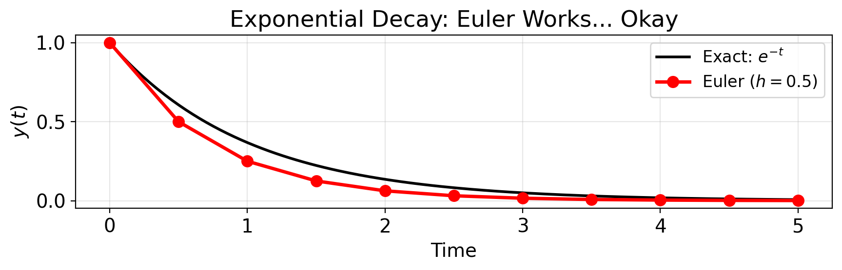

Time: 16-18 min. “Not perfect, but it tracks the solution. Euler looks fine here. Now let’s try something harder.”

Now the Real Test

Exponential decay is forgiving — the solution shrinks, so errors shrink too.

What happens when the solution oscillates and energy should be conserved?

Time: 18-19 min. Build anticipation before the failure.

SHO: Setting Up the Code

def f_sho(t, y):
    """Harmonic oscillator: y = [x, v], dy/dt = [v, -omega^2 * x]."""
    x, v = y[0], y[1]
    omega_sq = 1.0  # omega = 1
    return np.array([v, -omega_sq * x])

def euler_integrate(f, y0, t_span, h):
    """Euler integration returning arrays of (t, y)."""
    t_vals = [t_span[0]]
    y_vals = [np.array(y0, dtype=float)]
    while t_vals[-1] < t_span[1] - 1e-12:
        t, y = t_vals[-1], y_vals[-1]
        y_new = y + h * f(t, y)
        t_vals.append(t + h)
        y_vals.append(y_new)
    return np.array(t_vals), np.array(y_vals)

y0_sho = [1.0, 0.0]  # x(0) = 1, v(0) = 0

Time: 19-20 min. “Same structure as the decay example. The only difference is f_sho returns a 2-component array — the state vector.”

SHO: The Diagnostic

\[x(0) = 1, \quad v(0) = 0 \quad \Longrightarrow \quad x(t) = \cos(t), \quad v(t) = -\sin(t)\]

Our diagnostic — total energy should be constant:

\[E = \underbrace{\tfrac{1}{2}v^2}_{\text{kinetic}} + \underbrace{\tfrac{1}{2}\omega^2 x^2}_{\text{potential}} = \tfrac{1}{2}(v^2 + x^2) = 0.5 \quad \text{(for our ICs with } \omega = 1\text{)}\]

If \(E\) changes → the method is injecting or removing energy.

Time: 20-21 min. “Energy is the diagnostic. If it changes, the method is lying. This is the same diagnostic you’ll use in Project 2 with gravitational energy.”

The Beautiful Failure: Trajectory

h = 0.1; t_end = 20 * np.pi  # 10 periods
t_euler, y_euler = euler_integrate(f_sho, y0_sho, [0, t_end], h)

fig, ax = plt.subplots(figsize=(10, 3))
ax.plot(np.linspace(0, t_end, 2000), np.cos(np.linspace(0, t_end, 2000)),
        'k-', alpha=0.5, lw=1.5, label='Exact')
ax.plot(t_euler, y_euler[:, 0], 'r-', lw=1, label=f'Euler ($h={h}$)')
ax.set(xlabel='Time', ylabel='$x(t)$')
ax.legend()
plt.tight_layout()
plt.show()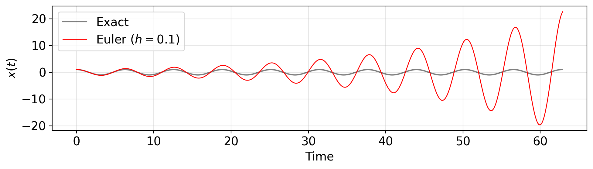

Time: 21-23 min. “Two things to see: (1) The amplitude is growing — that’s energy error, Euler is injecting energy. (2) The peaks are shifting — that’s phase error, Euler gets the timing wrong too. Both get worse with time.”

Phase Space Reveals the Crime

fig, ax = plt.subplots(figsize=(5, 4))
theta = np.linspace(0, 2 * np.pi, 200)
ax.plot(np.cos(theta), -np.sin(theta), 'k--', lw=2, label='Exact (circle)')
ax.plot(y_euler[:, 0], y_euler[:, 1], 'r-', lw=0.5, alpha=0.7,
        label='Euler (spiral)')
ax.set(xlabel='Position $x$', ylabel='Velocity $v$',
       title='Phase Space: Euler Spirals Outward')
ax.set_aspect('equal')
ax.legend()
plt.tight_layout()
plt.show()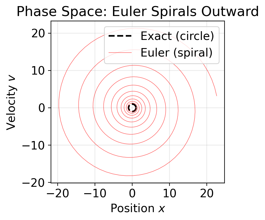

Time: 22-24 min. “The circle is the physical orbit in phase space. Euler spirals outward because every step overshoots — the tangent line always lands OUTSIDE the true circle.”

Energy Tells the Story

# Total energy: E = (1/2)(v^2 + omega^2 * x^2). For omega=1: E = (x^2 + v^2)/2
E_euler = 0.5 * (y_euler[:, 0]**2 + y_euler[:, 1]**2)

fig, ax = plt.subplots(figsize=(9, 3))
ax.plot(t_euler, E_euler, 'r-', lw=2, label='Euler')
ax.axhline(0.5, color='k', ls='--', lw=1.5, label='Exact ($E = 0.5$)')
ax.set(xlabel='Time', ylabel='Total Energy $E$',
       title='Energy Conservation: Euler FAILS')
ax.legend()
ax.set_ylim(0, min(E_euler[-1] * 1.1, E_euler[-1] + 50))
plt.tight_layout()
plt.show()

print(f"Energy at start: {E_euler[0]:.4f}")
print(f"Energy at end:   {E_euler[-1]:.1f}")
print(f"Energy grew by:  {(E_euler[-1] / E_euler[0] - 1) * 100:.0f}%")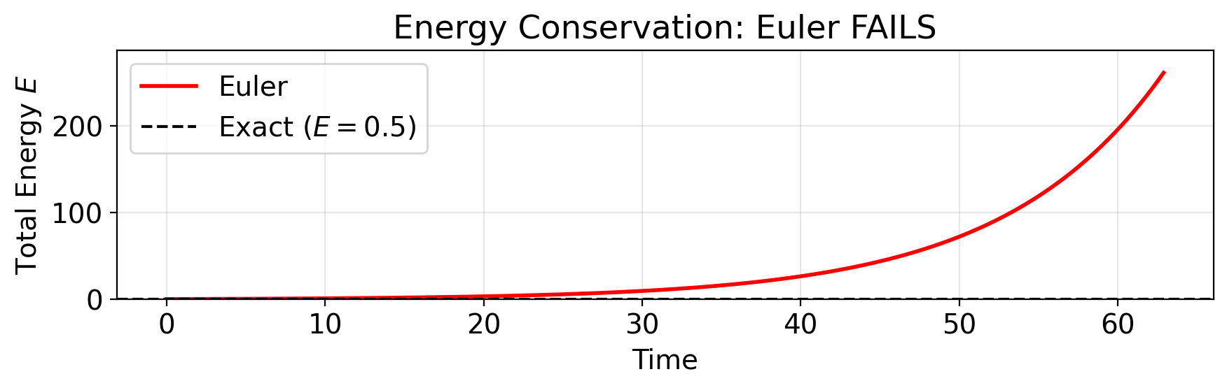

Energy at start: 0.5000
Energy at end:   261.3
Energy grew by:  52157%

Time: 24-26 min. “Energy grows exponentially. This is not a bug — it is a theorem about Euler on Hamiltonian systems.”

Why Euler Fails

Euler follows the tangent line at each point. For the oscillator, the true orbit curves inward (it’s a circle). The tangent is always outside the circle.

• Each step overshoots slightly
• The overshoot compounds — positive feedback
• Energy grows as \(E_n = E_0(1 + \omega^2 h^2)^n\)
• This is exponential growth in the step count \(n\)

Important

Making \(h\) smaller slows the growth but never stops it. Euler’s method on conservative systems is fundamentally broken.

(Euler is fine for non-oscillatory problems like exponential decay, and useful for first-pass debugging. The failure is specific to energy-conserving systems — which is exactly what Project 2 is.)

Time: 26-27 min. “The error is structural, not numerical. No amount of resolution fixes a structural flaw. We need a better method.”

From Equations to Code: RK2

The real skill: translating math into programs.

Time: 27-42 min. Core pedagogical section — equation-to-code translation.

Euler’s Problem, Visually

Euler uses the slope at the start of the interval and assumes it’s constant:

\[y_{n+1} = y_n + h \cdot f(t_n, y_n)\]

But the slope changes across the interval!

What if we could peek ahead to the middle and use a better slope estimate?

Time: 27-29 min. “Imagine walking through fog. Euler takes one look, walks straight for h steps. What if you could check your bearing at the midpoint?”

The Midpoint Method (RK2)

Step 1: Use Euler to estimate the state at the midpoint:

\[k_1 = f(t_n, y_n)\]

Step 2: Evaluate the slope at the midpoint:

\[k_2 = f\!\left(t_n + \frac{h}{2},\; y_n + \frac{h}{2}\,k_1\right)\]

Step 3: Use the midpoint slope for the full step:

\[\boxed{y_{n+1} = y_n + h \cdot k_2}\]

Local error: \(O(h^3)\). Global error: \(O(h^2)\). Second-order method. Cost: 2 evaluations per step.

Time: 29-32 min. “Three formulas. Each one becomes one line of code. Let’s do it.”

Equation to Code: Step by Step

The equations:

Math	Code
\(k_1 = f(t_n, y_n)\)	k1 = f(t, y)
\(k_2 = f(t_n + h/2,\; y_n + (h/2)\,k_1)\)	k2 = f(t + h/2, y + h/2 * k1)
\(y_{n+1} = y_n + h\,k_2\)	return y + h * k2

def rk2_step(f, t, y, h):
    """One step of RK2 (midpoint method): equations become code."""
    k1 = f(t, y)                          # slope at start
    k2 = f(t + h/2, y + h/2 * k1)        # slope at midpoint
    return y + h * k2                      # full step with better slope

Every symbol in the math has a one-to-one correspondence in the code.

This is the skill. RK4 and Leapfrog follow the exact same translation process.

Time: 32-35 min. “Walk through each line. Math left, code right. This is the core skill for Project 2.”

Full RK2 Integrator

def rk2_integrate(f, y0, t_span, h):
    """RK2 integration — same structure as euler_integrate."""
    t_vals = [t_span[0]]
    y_vals = [np.array(y0, dtype=float)]
    while t_vals[-1] < t_span[1] - 1e-12:
        t, y = t_vals[-1], y_vals[-1]
        y_new = rk2_step(f, t, y, h)     # <-- only this line changes!
        t_vals.append(t + h)
        y_vals.append(y_new)
    return np.array(t_vals), np.array(y_vals)

Compare with euler_integrate — the only difference is calling rk2_step instead of computing y + h * f(t, y) directly.

The integration loop is method-agnostic. Swap the step function, get a different method.

Time: 35-36 min. “This design pattern is powerful. You’ll use the same loop structure for RK4 and Leapfrog.”

Why Should RK2 Be Better?

Recall the Taylor series: \(\;y(t+h) = y + hy' + \frac{h^2}{2}y'' + \frac{h^3}{6}y''' + \cdots\)

• Euler matches the first 1 term (\(h\)). Everything from \(h^2\) onward is error.
• RK2 matches the first 2 terms (\(h\) and \(h^2\)). Error starts at \(h^3\).
• Each additional matched term pushes the leading error to a higher power of \(h\).
• Since \(h < 1\) (typically \(h \approx 0.01\)), higher powers shrink fast: \(0.01^2 = 10^{-4}\), \(0.01^4 = 10^{-8}\).

Tip

The recipe for accuracy: Sample the slope at more points → match more Taylor terms → push the error to a higher power of \(h\). That’s the entire Runge-Kutta idea.

Let’s verify this prediction…

Time: 36-37 min. “This is the deep reason. Now let’s see if the prediction holds.”

RK2 vs Euler: Trajectory

t_rk2, y_rk2 = rk2_integrate(f_sho, y0_sho, [0, t_end], h)

fig, ax = plt.subplots(figsize=(10, 3))
ax.plot(t_exact, np.cos(t_exact), 'k-', alpha=0.4, lw=1.5, label='Exact')
ax.plot(t_euler, y_euler[:, 0], 'r-', lw=0.8, alpha=0.5, label='Euler')
ax.plot(t_rk2, y_rk2[:, 0], 'b-', lw=1.5, label='RK2')
ax.set(xlabel='Time', ylabel='$x(t)$',
       title='RK2 vs Euler: Night and Day')
ax.legend()
plt.tight_layout()
plt.show()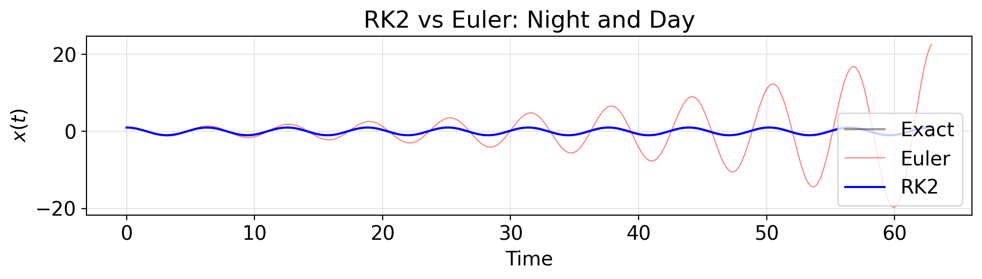

Time: 36-38 min. “RK2 tracks the solution far better. Two evaluations per step instead of one — and we go from first-order to second-order.”

RK2 vs Euler: Phase Space

fig, (ax1, ax2) = plt.subplots(1, 2, figsize=(11, 3.5))
theta = np.linspace(0, 2 * np.pi, 200)

ax1.plot(np.cos(theta), -np.sin(theta), 'k--', lw=2)
ax1.plot(y_euler[:, 0], y_euler[:, 1], 'r-', lw=0.3, alpha=0.6)
ax1.set(title='Euler: Spiral Out', xlabel='$x$', ylabel='$v$')
ax1.set_aspect('equal')

ax2.plot(np.cos(theta), -np.sin(theta), 'k--', lw=2)
ax2.plot(y_rk2[:, 0], y_rk2[:, 1], 'b-', lw=0.5, alpha=0.7)
ax2.set(title='RK2: Much Tighter', xlabel='$x$', ylabel='$v$')
ax2.set_aspect('equal')

plt.tight_layout()
plt.show()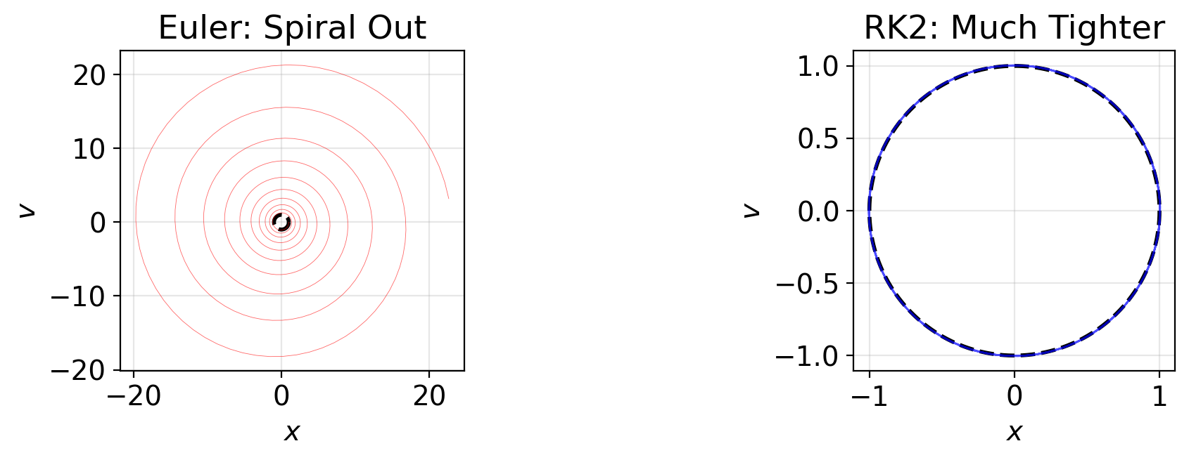

Time: 38-39 min. “RK2’s orbit stays much closer to the circle. But zoom in — it still drifts. Can we do even better?”

RK2 vs Euler: Energy

E_rk2 = 0.5 * (y_rk2[:, 0]**2 + y_rk2[:, 1]**2)

fig, (ax1, ax2) = plt.subplots(1, 2, figsize=(12, 3))

# Left: both on same scale
ax1.plot(t_euler, E_euler, 'r-', lw=1.5, label='Euler')
ax1.plot(t_rk2, E_rk2, 'b-', lw=1.5, label='RK2')
ax1.axhline(0.5, color='k', ls='--', lw=1)
ax1.set(xlabel='Time', ylabel='Energy $E$', title='Full Scale')
ax1.legend()

# Right: zoom on RK2
ax2.plot(t_rk2, E_rk2 - 0.5, 'b-', lw=1.5)
ax2.axhline(0, color='k', ls='--', lw=1)
ax2.set(xlabel='Time', ylabel='$E - E_0$', title='RK2 Energy Error (Zoomed)')

plt.tight_layout()
plt.show()

print(f"Euler final energy error: {abs(E_euler[-1] - 0.5):.1f}")
print(f"RK2 final energy error:   {abs(E_rk2[-1] - 0.5):.2e}")
print(f"RK2 is {abs(E_euler[-1] - 0.5) / abs(E_rk2[-1] - 0.5):.0f}x better")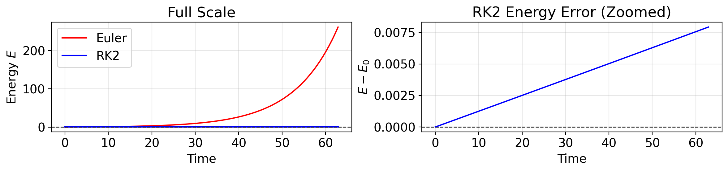

Euler final energy error: 260.8
RK2 final energy error:   7.92e-03
RK2 is 32908x better

RK2 is vastly better. But it still drifts. Over millions of timesteps — the kind you’ll run for Project 2 — that drift adds up. Is there something better?

Time: 39-42 min. “RK2 reduced the error by orders of magnitude. But zoom in — it still drifts monotonically. For a million-step simulation, we need methods that preserve energy exactly.”

Higher-Order Methods: Your Turn

Now you have the skill. Apply it.

Time: 42-52 min. Show formulas, don’t code — students implement for Project 2.

RK4: Four Slopes, Fourth-Order

\[k_1 = f(t_n,\, y_n)\] \[k_2 = f\!\left(t_n + \tfrac{h}{2},\; y_n + \tfrac{h}{2}\,k_1\right)\] \[k_3 = f\!\left(t_n + \tfrac{h}{2},\; y_n + \tfrac{h}{2}\,k_2\right)\] \[k_4 = f(t_n + h,\; y_n + h\,k_3)\]

\[\boxed{y_{n+1} = y_n + \frac{h}{6}\left(k_1 + 2k_2 + 2k_3 + k_4\right)}\]

Matches Taylor series through \(h^4\) — error starts at \(h^5\).

Halve \(h\)	Error drops by
Euler (\(p=1\))	\(2\times\)
RK2 (\(p=2\))	\(4\times\)
RK4 (\(p=4\))	\(16\times\)

Same pattern as RK2 — each \(k\) formula becomes one line of code.

Weights \(\frac{1}{6}, \frac{2}{6}, \frac{2}{6}, \frac{1}{6}\) are Simpson’s rule!

Time: 44-46 min. “4 evaluations per step, but each halving of h gives 16x improvement. The Simpson’s rule connection is deep — RK4 is doing numerical integration of the slope function.”

The Problem With All Runge-Kutta Methods

RK2, RK4, even RK8 — they all share a fundamental flaw:

• They treat \([x, v]\) as a single blob and update everything at once
• This is accurate locally but violates a deep physical principle
• Liouville’s theorem: physical systems preserve phase space volume
• RK methods shrink or expand phase space slightly each step
• Over millions of steps: systematic energy drift (always in the same direction)

Warning

No amount of accuracy fixes a structural violation. We need a method that respects the geometry of physics.

Time: 46-48 min. “This is the deepest idea in the lecture. Accuracy and structure are different things. You can be very accurate and still violate physics.”

Leapfrog: Structure Over Accuracy

A fundamentally different idea: update position and velocity alternately, not simultaneously.

Kick-Drift-Kick:

\[\vec{v}_{n+1/2} = \vec{v}_n + \frac{h}{2}\,\vec{a}(\vec{r}_n) \qquad \text{(half kick)}\]

\[\vec{r}_{n+1} = \vec{r}_n + h\,\vec{v}_{n+1/2} \qquad \text{(full drift)}\]

\[\vec{v}_{n+1} = \vec{v}_{n+1/2} + \frac{h}{2}\,\vec{a}(\vec{r}_{n+1}) \qquad \text{(half kick)}\]

Time: 48-49 min.

Why Leapfrog Preserves Energy

Each sub-step is a shear — stretches phase space in one direction but preserves total area:

• Kick: changes velocity, leaves position alone → shear in \(v\)-direction
• Drift: changes position, leaves velocity alone → shear in \(x\)-direction
• Shears preserve area exactly (like pushing a deck of cards sideways)
• Composition of area-preserving maps = area-preserving map

Result: Leapfrog conserves a slightly modified energy \(\tilde{E} = E + O(h^2)\).

• \(\tilde{E}\) is conserved exactly → energy oscillates within a bounded envelope
• The envelope width is \(\propto h^2\) → shrinks with smaller timestep
• Energy never drifts — bounded forever, no matter how many steps

Property	RK4	Leapfrog
Order	4th	2nd
After \(10^6\) steps	Drifts by \(\sim 0.1\%\)	Oscillates within \(\sim 0.01\%\)
After \(10^9\) steps	Drifts by \(\sim 100\%\)	Still within \(\sim 0.01\%\)

Important

Only 2nd order — but energy is conserved to machine precision. Structure preservation beats raw accuracy.

Time: 49-52 min. “This is the key insight. A deck of cards pushed sideways doesn’t change in area. Three shears composed = area preserved = energy bounded. A 2nd-order method that preserves physics beats a 4th-order method that doesn’t.”

Your Turn: RK4

Formulas

\[k_1 = f(t_n, y_n)\] \[k_2 = f(t_n + \tfrac{h}{2}, y_n + \tfrac{h}{2}k_1)\] \[k_3 = f(t_n + \tfrac{h}{2}, y_n + \tfrac{h}{2}k_2)\] \[k_4 = f(t_n + h, y_n + hk_3)\] \[y_{n+1} = y_n + \tfrac{h}{6}(k_1 + 2k_2 + 2k_3 + k_4)\]

Your Code

def rk4_step(f, t, y, h):
    k1 = ???
    k2 = ???
    k3 = ???
    k4 = ???
    return ???

Same pattern as RK2 — each \(k\) formula becomes one line.

Time: 52-53 min. “You practiced this with RK2. Each formula maps to one line of code.”

Your Turn: Leapfrog

Formulas (Kick-Drift-Kick)

\[v_{n+1/2} = v_n + \tfrac{h}{2}\,a(x_n)\] \[x_{n+1} = x_n + h\,v_{n+1/2}\] \[v_{n+1} = v_{n+1/2} + \tfrac{h}{2}\,a(x_{n+1})\]

where \(a(x) = -\omega^2 x\) (or \(= F/m\) for gravity)

Your Code

def leapfrog_step(x, v, a_func, h):
    v_half = ???      # half kick
    x_new  = ???      # full drift
    a_new  = ???      # force at new position
    v_new  = ???      # half kick
    return x_new, v_new

Notice: Leapfrog takes \((x, v)\) separately — not a single state vector.

This structural difference is why it preserves energy.

Time: 53-54 min. “Leapfrog has a different API. It updates x and v separately, not as one vector. That’s the whole point — the alternating structure is what makes it symplectic.”

Method Comparison

Method	Order	Energy Behavior	Symplectic?	Evals/Step	Best For
Euler	1st	Exponential growth	No	1	Learning
RK2	2nd	Moderate drift	No	2	Quick tests
RK4	4th	Slow drift	No	4	Short-time accuracy
Leapfrog	2nd	Bounded oscillation	Yes	1*	Long-time dynamics

* Leapfrog reuses the last acceleration, so effectively 1 new evaluation per step.

For Project 2, you’ll implement three of these (Euler, RK4, Leapfrog) and discover these differences yourself.

Time: 50-52 min. “This table summarizes the whole lecture. You should be able to explain every entry by the time you finish Project 2.”

Project 2: N-body Dynamics

Time: 52-60 min. Project launch.

The Challenge

Build a gravitational N-body simulator from scratch.

• Build the complete pipeline with Euler first (force calc → integration → diagnostics → plots)
• Add RK4 and Leapfrog as drop-in replacements — compare energy behavior
• Generate Plummer sphere initial conditions for realistic star clusters
• Compare loops vs. vectorized NumPy (\(10\)–\(100\times\) speedup)

Time: 52-54 min. “The key idea: build one working pipeline first, then upgrade pieces. Phase 1 is all about getting Euler working end-to-end.”

The Pipeline-First Approach

Phase	What You Build	What You Validate
1	Euler pipeline (\(N=2\), \(N=3\))	Force calc, energy diagnostics, plotting
2	Add RK4 + Leapfrog	Integrator comparison on same \(N=2\) problem
3	Plummer sphere ICs (\(N=10\)–\(100\))	Virial equilibrium, cluster dynamics
4	Vectorized forces (\(N=1000+\))	Performance scaling, loop vs. NumPy

Tip

Each phase adds one new idea on top of a validated foundation. Phase 1 is the hardest — once your pipeline works end-to-end, everything else is incremental.

Time: 54-56 min. “Phase 1 is your priority this week. Get Euler working end-to-end on a Sun-Earth orbit. The rest builds on that foundation.”

What You Should Observe

Today’s harmonic oscillator = tomorrow’s gravitational orbit:

• Euler will spiral your planet outward until it escapes — just like our spring
• RK4 will produce nearly perfect orbits with tiny drift
• Leapfrog will keep energy bounded with no drift — orbits stay closed forever

The physics is different (gravity vs. spring), but the numerical behavior is identical.

“Today’s spring = tomorrow’s gravity.”

Time: 56-57 min. “This connection is the whole point. Same math, same methods, same failure modes.”

Timeline and Milestones

• Check-in 1 (Wed Feb 18): Phase 1 complete — Euler pipeline working end-to-end, \(N=2\) orbit plot, energy diagnostics. At least 3 meaningful commits.
• Check-in 2 (Wed Feb 25): Phase 2 complete — all three integrators compared on \(N=2\), energy error plot. Phase 3 started (Plummer ICs).
• Due: Tue Mar 3, 11:59 PM. Phases 3–4 complete — cluster simulations, vectorization, all plots, both memos.

Time: 57-58 min. “Check-in 1 is the critical one. If you can’t get Euler working on a Kepler orbit by next Wednesday, come to office hours immediately.”

Reading Assignments

Before next class, read these from the course website:

• Module 3, Part 1: Failure of Naive Integration — full Euler derivation, error analysis
• Module 3, Part 2: Runge-Kutta Methods — complete RK4 derivation, adaptive stepping
• Module 3, Part 3: Symplectic Integration — Hamiltonian mechanics, Leapfrog, phase space

The Takeaway

Structure > Accuracy

Time: 58-60 min. “Today you saw the failure. The readings explain WHY it fails mathematically. By next class, you should be coding Phase 1 — get Euler running on a Sun-Earth orbit.”