Learning Objectives
By the end of this section, you will be able to:
Implement bisection, Newton-Raphson, and secant methods from scratch
Analyze convergence rates (linear, superlinear, quadratic) mathematically
Diagnose method failures and design robust hybrid approaches
Apply root finding to Kepler’s equation, Lagrange points, and stellar structure
Predict iteration counts and verify convergence behavior
The Fundamental Problem
Root/Zero: A value where . The x-intercept of the function. In physics, often represents equilibrium points.
Transcendental equation: An equation involving transcendental functions such as sine, exponential, or logarithm. Many require numerical solution, but some have explicit solutions: gives .
In physics, equilibrium occurs where the net force vanishes, where a differentiable potential energy is stationary, or where competing effects balance. Mathematically, these all reduce to finding roots of equations: solving .
Many equations in computational physics have no closed-form solution. For example, a stellar model must satisfy hydrostatic equilibrium:
This is a differential equation, not itself a scalar root equation. Once we discretize a stellar model or impose a boundary condition, root finding can determine an unknown central value, radius, or model parameter. We need to distinguish solving the ODE from solving that resulting residual equation.
Root sensitivity: For a simple scalar root , describes the sensitivity to an additive perturbation in the function value. Its numerical meaning depends on the chosen units and on the error model.
Building Intuition: The Geometry of Root Finding
Before diving into algorithms, let’s understand the geometry. Finding roots is about locating zeros; a curve can cross the x-axis or touch it without crossing. Different methods use different geometric insights:
Bracketing: Maintaining an interval whose endpoint values have opposite signs. If the function is continuous on that interval, the Intermediate Value Theorem guarantees at least one root inside.
Interpolation: Approximating a function between known points using simpler functions (lines, parabolas, etc.).
Bracketing methods (bisection) maintain an interval with a sign change.
Local methods (Newton) use a tangent-line model near an iterate.
Interpolation methods (secant) replace the analytic derivative with a slope from two evaluations.
Each approach has trade-offs between:
Reliability: Will it always find a root?
Speed: How many iterations to converge?
Requirements: Do we need derivatives? Good initial guesses?
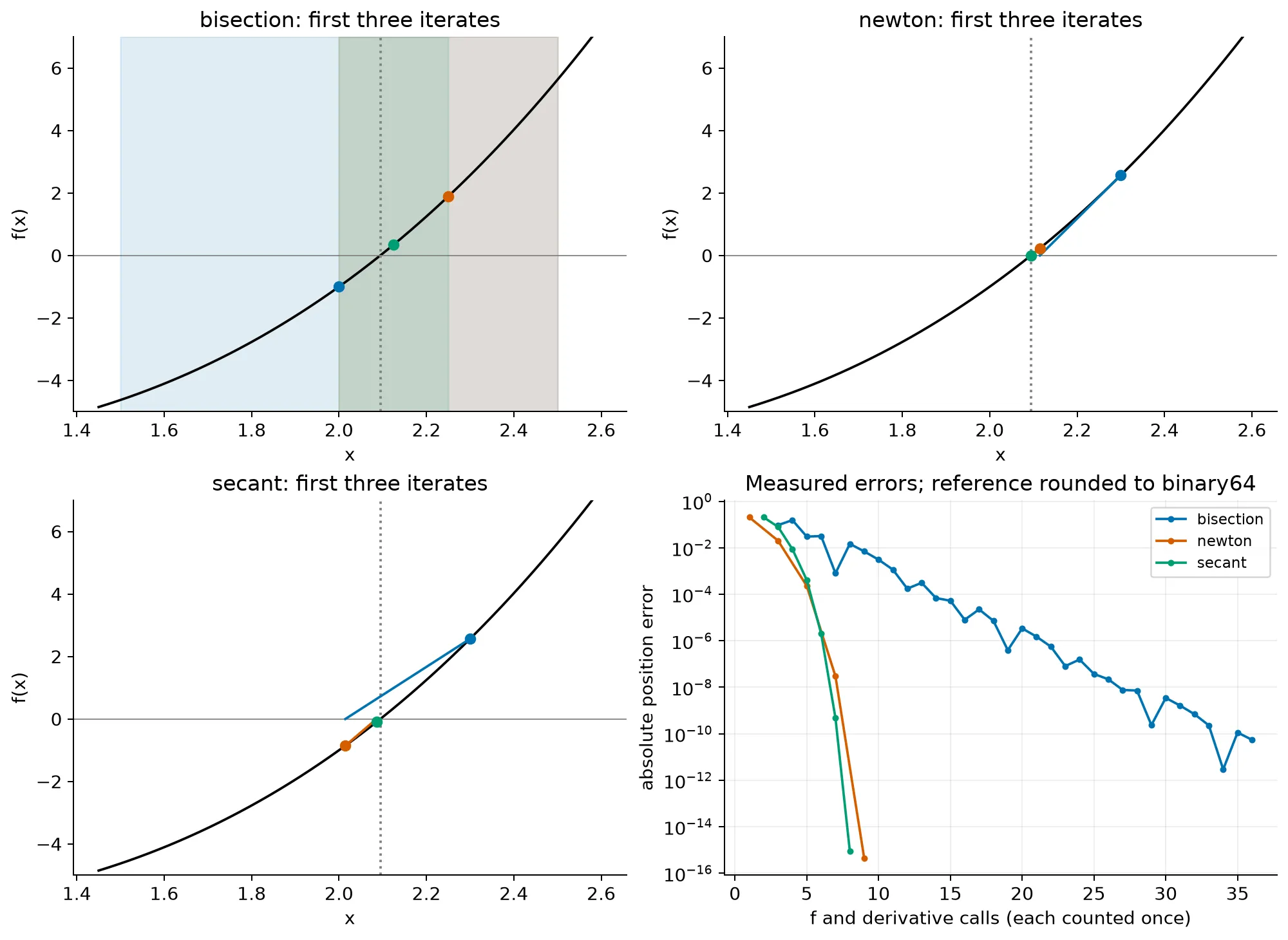
Figure 1:Root-finding geometry for . Bisection starts on , Newton at 2.3, and secant with 1.5 and 2.3. The first three iterates show how each method obtains its next position. The fourth panel compares errors against a reference bracketed in 70-digit decimal arithmetic, then rounded to binary64. The horizontal axis counts function and derivative calls separately, with one unit for each; these calls need not have equal runtime. Bracket half-width tolerance is 10-10 and the cap is 40 iterations. Zero computed residuals and floating-point stagnation end a run. Zero plotted errors are omitted, not replaced by an invented floor.
Method 1: Bisection
The Mathematical Foundation
Intermediate Value Theorem: If is continuous on and is any value between and , then there exists at least one where . Strictly intermediate values occur in the open interval.
The bisection method is based on the Intermediate Value Theorem:
If is continuous on and , then there exists at least one root where .
The algorithm repeatedly halves the interval, keeping the half that contains the root.
Algorithm Analysis
Starting with interval where :
Compute midpoint:
Evaluate
Update interval:
If : return the sampled zero; otherwise stop only when the half-width meets the requested position tolerance
If : root in , so set ,
Otherwise: root in , so set ,
After iterations, the interval width is:
Linear convergence of the bound: Bisection halves its bracket half-width at each update. Its actual midpoint error need not decrease by exactly one half, or even decrease at every update.
The error in our approximation is bounded by half the interval width:
This is linear convergence with rate .
Iterations Required
To achieve error , we need:
Solving for :
For example, to find a root in to 10 decimal places ():
So 33 interval halvings suffice, followed by the new midpoint, provided continuity and reliable function signs hold. Count midpoint evaluations separately from interval updates.
Implementation
This reading uses a compact reference interface to illustrate bracket reduction. It differs from the Project 3 contract:
| Reading example | Project 3 |
|---|---|
bisection(..., tol=...) returns one scalar | bisect(..., atol=..., rtol=...) returns (root, n_iter, history) |
An exact sampled root may be passed as (x, x) | Require a < b; retain exact sampled roots separately |
| Absolute position tolerance only | Absolute plus relative position allowance |
Use the project brief for submitted interfaces, history recording, and failure behavior. The example below is a reading reference, not a replacement module.
import math
import numpy as np


def bisection(f, a, b, tol=1e-10, max_iter=100):
    """Return a bracket midpoint with absolute position tolerance tol.

    f must be continuous, finite, scalar-valued, and reliably signed.
    tol has x's units; it is not a tolerance on the residual f(x).
    """
    if not (math.isfinite(a) and math.isfinite(b) and a <= b):
        raise ValueError("Need finite ordered endpoints")
    if not math.isfinite(tol) or tol <= 0:
        raise ValueError("tol must be positive and finite")
    if isinstance(max_iter, (bool, np.bool_)) or not isinstance(max_iter, (int, np.integer)) or max_iter <= 0:
        raise ValueError("max_iter must be a positive integer")

    def evaluate(x):
        value = float(f(x))
        if not math.isfinite(value):
            raise ValueError("f must return finite values")
        return value

    fa, fb = evaluate(a), evaluate(b)
    if fa == 0.0:
        return a
    if fb == 0.0:
        return b
    # Comparing signs avoids overflow/underflow from multiplying values.
    if (fa < 0) == (fb < 0):
        raise ValueError("Need opposite signs at the endpoints")

    for _ in range(max_iter):
        c = a / 2 + b / 2   # Avoid overflow in a + b.
        if max(c - a, b - c) <= tol:
            return c
        if c == a or c == b:
            raise RuntimeError("No representable interior point; tolerance unmet")
        fc = evaluate(c)
        if fc == 0.0:
            return c
        if (fa < 0) != (fc < 0):
            b, fb = c, fc
        else:
            a, fa = c, fc
    raise RuntimeError(f"Failed to converge in {max_iter} iterations")
An exactly zero computed function value is accepted here. If evaluating the function can underflow to zero or produce unreliable signs, the bracket is no longer certified by these values. Rescale the evaluation or use higher precision; changing the stopping criterion cannot repair the function evaluation.
Predict → Run → Explain: small residual or well-located root?
Multiplying a function by a positive constant does not move its root. Predict whether the same position tolerance should give the same answer for both rows.
for scale in (1.0, 1e-12, 1e-200):
    f_scaled = lambda x: scale * (x - 0.9)
    root = bisection(f_scaled, 0.0, 1.0, tol=1e-10)
    print(f"scale={scale:.0e}: root={root:.12f}, "
          f"position error={abs(root-0.9):.3e}, residual={abs(f_scaled(root)):.3e}")
scale=1e+00: root=0.899999999965, position error=3.492e-11, residual=3.492e-11
scale=1e-12: root=0.899999999965, position error=3.492e-11, residual=3.492e-23
scale=1e-200: root=0.899999999965, position error=3.492e-11, residual=3.492e-211
The position errors agree although the residuals differ by many orders of magnitude. Near a simple root, : a residual measures position error only after accounting for the slope and the function’s units. If on the relevant interval, the mean value theorem gives . A bracket gives a position bound without estimating that slope.
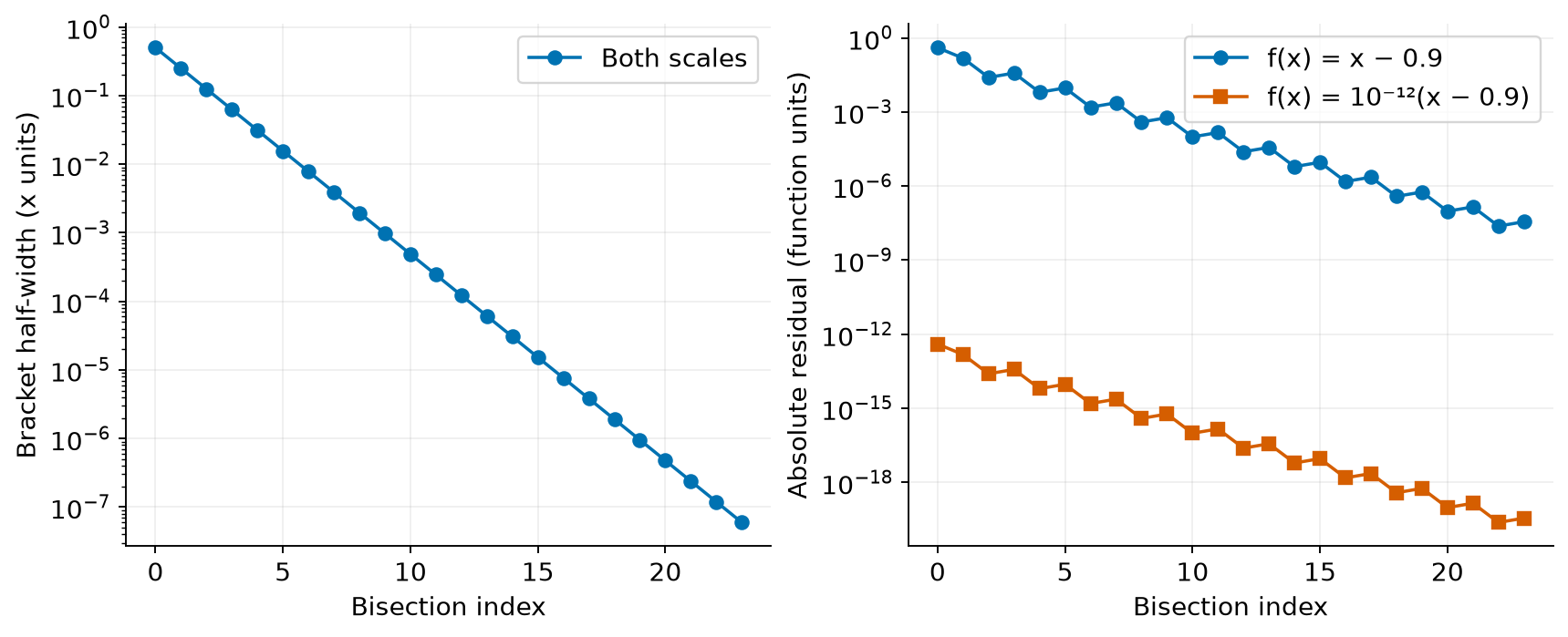
Both functions have root 0.9 and use the same sequence of brackets. Residual size depends on the vertical scale; bracket width measures uncertainty in x.
Common Failure Modes and Fixes
| Problem | Symptom | Solution |
|---|---|---|
| No sign change | Won’t start | Scan interval for brackets first |
| Multiple roots | Finds arbitrary one | Use smaller initial intervals |
| Discontinuity | False bracket | Check continuity requirement |
| touches zero | No sign change | Bisection cannot certify this root; use a method with different assumptions or bracket a related sign-changing quantity |
Answers and reasoning
Opposite signs plus continuity establish at least one crossing. Compare signs in code instead of multiplying tiny values.
The interval may contain several roots; bisection narrows toward a crossing without identifying which physical root you intended.
A sampled zero can be returned, but an even-multiplicity root without a sign change cannot be certified by a surrounding bisection bracket.
For absolute position error below 10-6, requires interval halvings, followed by that bracket’s midpoint. The first midpoint is index zero; count evaluations separately.
Method 2: Newton-Raphson — using a local slope
The Geometric Insight
Tangent line approximation: Replacing a curve with its tangent line at a point, valid for small deviations.
Newton’s method uses calculus to accelerate convergence. The key insight: near any point, a smooth function looks approximately linear. We follow the tangent line to where it crosses the axis. Sufficiently near a simple root, under suitable smoothness conditions, this can provide a much more accurate estimate. A tangent step from an arbitrary starting point need not improve the estimate.
Mathematical Derivation
Starting at point , the tangent line to has equation:
This line crosses the x-axis (where ) at:
Solving for :
This is the Newton-Raphson iteration formula.
Convergence Analysis
To understand the convergence rate, we analyze the error where is the true root.
Using Taylor series around :
Since :
Similarly:
Through algebraic manipulation of the Newton iteration formula:
Quadratic convergence: Error is squared each iteration, doubling the number of correct digits.
For a sufficiently smooth function, a simple root with , and a sufficiently close initial guess, this shows quadratic convergence! The error is squared each iteration, meaning the number of correct digits approximately doubles.
When Newton Fails
The tangent model can fail for several distinct reasons:
Zero derivative away from a root: If and , the horizontal tangent has no zero
Poor initial guess: May diverge or converge to wrong root
Cycles: Can oscillate between points without converging
Sensitive root: A small amplifies a given absolute function error; interpret that error together with units and function scaling
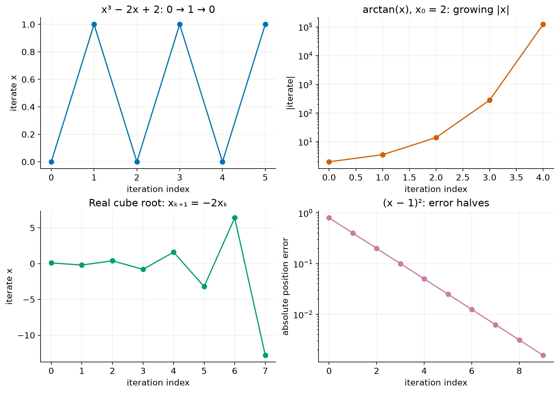
Figure 3:Four directly computed Newton histories isolate different mechanisms. For , the initial value 0 cycles exactly between 0 and 1. For , starting at 2 gives rapidly growing iterate magnitudes. For the real cube root, every nonzero iterate obeys ; the derivative is undefined at the root, and starting nearby does not help. For , Newton halves the position error rather than squaring it. These are separate failure or convergence mechanisms; a small derivative at an arbitrary iterate is not the same thing as a sensitive root.
Common Failure Modes and Fixes
| Problem | Symptom | Solution |
|---|---|---|
| f’(x) 0 | Division by small number | Use bisection if a valid sign-changing bracket is available |
| Bad initial guess | Divergence | Find and verify a sign-changing bracket, then use bisection |
| Oscillation | Repeating values | Detect cycles, switch methods |
| Repeated root | Slow convergence | Use modified Newton: |
Method 3: Secant - The Practical Compromise
Motivation: No Derivatives Required
Finite difference approximation: Estimating derivatives using function values at nearby points.
Newton’s method requires , but what if:
The derivative is expensive to compute?
We only have as a black box?
The function comes from experimental data?
The secant method approximates the derivative using a finite difference:
The Iteration Formula
Substituting this approximation into Newton’s formula:
Geometrically, we’re replacing the tangent line with a secant line through two points.
Convergence Analysis
For a sufficiently smooth function with a simple root and sufficiently close starting points, the convergence of the secant method is more complex. Through detailed analysis (involving difference equations), one can show that the order of convergence is:
This is the golden ratio! The error satisfies:
Superlinear convergence: as the root is approached. Quadratic convergence is also superlinear; secant convergence is specifically superlinear and subquadratic.
This superlinear convergence is slower than Newton’s quadratic rate but faster than bisection’s linear rate.
Where the golden ratio comes from
The secant slope contains information from two previous errors. Expanding , with and , gives
Substituting in the secant update and cancelling the leading linear term gives
Suppose this nonzero leading term controls the iteration and the errors obey . Then scales like , so
Thus , and the positive root is . The result comes from reusing two iterates, not from a universal empirical ranking of solvers. If the leading coefficient vanishes, the root is repeated, or rounding dominates, this particular asymptotic calculation does not describe the measured sequence.
Answer: an order is not a timing result
Count the work needed to reach the same justified error target, including initialization and failed steps. Newton may need fewer iterations but more expensive evaluations. The local order describes an asymptotic error relation; it does not supply the constants, basin of convergence, or runtime of an application’s derivative calculation.
Comparison of Convergence Rates
| Method | Order | Error Reduction | Digits Gained/Iteration | Function Evals |
|---|---|---|---|---|
| Bisection | 1.0 (bound) | Half-width halves; actual error need not | About 0.30 in the bound | 1 |
| Secant | 1.618 | Correct-digit count grows by roughly 1.618 | 1 new, after initialization | |
| Newton | 2.0 | Doubles | 2 (f and f’) |
The bracket bound can contract even when successive midpoint errors do not. The computed example below uses ; it compares actual errors with the bisection bound, not with residuals or update sizes.
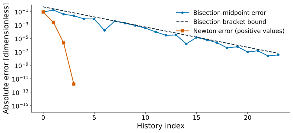
The measured midpoint error can rise while its guaranteed bracket bound falls. Zero error cannot be displayed on a logarithmic axis.
There is no universal absolute cutoff for a “small” secant denominator: multiplying the equation by a constant scales that denominator while leaving the exact secant step unchanged. Compare evaluation uncertainty with the local function-value scale and inspect the proposed step. If function error dominates the difference, report an unreliable slope or use a justified safeguard. Project 3 requires explicit handling of zero denominators and nonfinite values; it does not prescribe an extra arbitrary near-zero threshold.
Common Failure Modes and Fixes
| Problem | Symptom | Solution |
|---|---|---|
| f(x₀) f(x_{1}) | Near-zero denominator | Report an unusable slope; restart with justified points or use a bracketed safeguard |
| Parallel secants | No convergence | Restart with different points |
| Leaves bracket | May miss root | Use a bracket-preserving hybrid; Brent is one specific algorithm, not any secant/bisection combination |
Answers and reasoning
Secant needs function values but no analytic derivative.
Near a smooth simple root its two-point error recurrence gives superlinear order about 1.618. Newton uses derivative information to reach quadratic order; bisection instead guarantees a halving bracket bound.
Two previous points and their function values; after initialization, only one new function value is needed per update.
Secant is useful when derivatives are expensive and starting points are credible. If maintaining a bracket is essential, use a safeguarded method rather than assuming secant retains it.
Backtracking: choose how far to follow Newton
Newton proposes a direction . A line search chooses a step length along that direction:
The full Newton step uses . Backtracking starts there and shortens the step when it fails an acceptance test. This controls a local proposal; it does not preserve a root bracket or select a physically meaningful root.
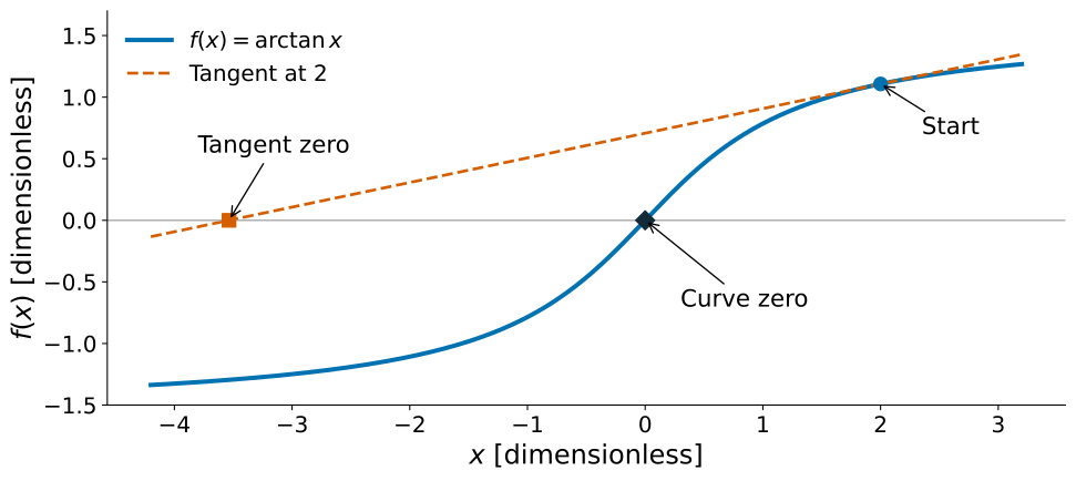
Newton finds the zero of a local tangent. That proposal still needs an actual function evaluation before it can be accepted.
Define progress before testing a step
For a scalar equation, use the merit function . With a differentiable and finite nonzero , an exact Newton direction satisfies
at a nonroot. It is a descent direction locally, although a full step can increase the merit function. The Armijo sufficient-decrease test is
Choose here; the example uses and halves after each rejection. These are illustrative algorithm settings, not accuracy tolerances. Under the differentiability and descent assumptions, sufficiently small positive steps satisfy this test in exact arithmetic. A finite search budget, floating-point stagnation, or unreliable evaluations can still prevent an implementation from accepting a step.
Predict, compare, explain: one accepted step
For , start at . Predict whether the full Newton step reduces , then compare these candidate trials (including an extra quarter-step for comparison). This is one step, not a complete solve.
| Step fraction | Trial | Residual magnitude | Armijo test |
|---|---|---|---|
| 1 | -3.535744 | 1.295169 | Reject |
| -0.767872 | 0.654841 | Accept | |
| 0.616064 | 0.552148 | Accept |
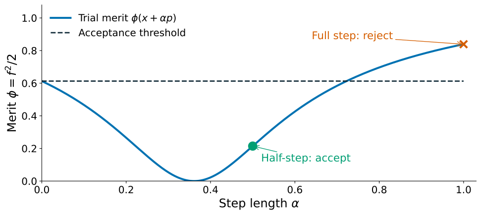
The acceptance test compares the actual merit value with the sufficient-decrease threshold. The quarter-step is shown only to compare candidates; an ordinary backtracking search would stop at the accepted half-step.
Backtracking accepts the first passing trial, not necessarily the best point on the line. Explain why an accepted step neither identifies a root nor preserves a bracket. No line-search implementation is assigned.
The full step reaches approximately −3.536 and increases the residual magnitude. One halving reaches approximately −0.768 and satisfies sufficient decrease. This is progress, not a converged root. A complete solver still needs an outer iteration budget, stopping rules, diagnostics, and a physical-domain check. Domain-restricted functions also need an explicit feasible-trial policy; this example does not turn arbitrary domain errors into successful steps.
Three different ways to control a proposal
| Approach | What it controls | What it does not establish by itself |
|---|---|---|
| Backtracking line search | Distance along a direction, using sufficient decrease | A root-error bound, a bracket, or the physical root |
| Bracket-preserving hybrid | Proposed steps plus reliable bracket reduction | Continuity or correctness of supplied function signs |
| Levenberg regularization | The linear system that defines the direction | A zero residual or a globally successful solve |
FNC’s quasi-Newton chapter develops Levenberg’s method for nonlinear systems: regularization changes the proposed step, and residual reduction governs acceptance. It is related to step control but is not the scalar backtracking algorithm above. For a production Newton/line-search interface, see PETSc. Levenberg’s method is a preview for later nonlinear least squares, not another algorithm to implement this week.
Jacobians and local fitting · Week 5 companion
For observations and a model , define residuals . With observations and parameters, the Jacobian has shape and entries . Each row describes one observation; each column describes sensitivity to one parameter.
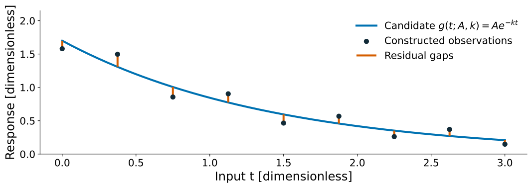
Changing either parameter changes several residuals at once. These points are constructed for illustration, not measured data or the three-point Jacobian example that follows.
For a small parameter update , . The product predicts a change, not the new residual itself.
For at , , and (scaled, dimensionless coordinates),
The update predicts changes . Actual changes are approximately . Reducing the step by ten reduces the largest discrepancy by about 99: the linear approximation improves locally.
The least-squares loss is , where . Transpose, written , exchanges rows and columns. The loss gradient (its parameter partial derivatives) is .
Gauss–Newton minimizes . A Levenberg step adds a penalty on the current update:
Setting gives
Here is the identity matrix and controls damping. The parameters must be scaled sensibly; Marquardt variants incorporate scaling. This is a penalty on an update, not a fixed prior on the parameters. Check actual loss reduction before accepting a trial. The displayed normal equations explain the method; production solvers can use QR or SVD to avoid the conditioning penalty of explicitly forming .
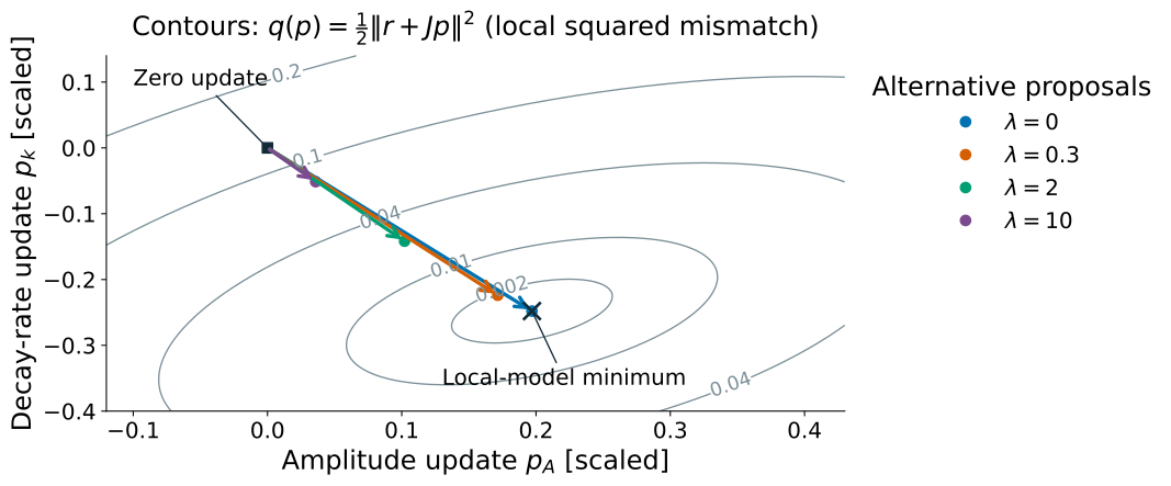
Contours show the local squared-residual model in scaled parameter updates. Each arrow starts at zero and represents a different damping choice, not the next point of one trajectory. Actual loss must be checked separately.
In regression and calibration, noisy data generally cannot all have zero residual. This differs from solving a square system , where a nonsingular (invertible) Jacobian gives the Newton proposal . Damping can control a poor step but cannot create information absent from the observations. For example, early observations of a decay curve weakly constrain because is small near .
Explain: why can a tiny damped step coexist with a large residual? No implementation of these advanced fitting methods is required for Project 3.
Hybrid Methods: preserve a bracket while using local models
A safeguarded method uses interpolation or a derivative when the proposed step is acceptable and falls back to bracket reduction when it is not.
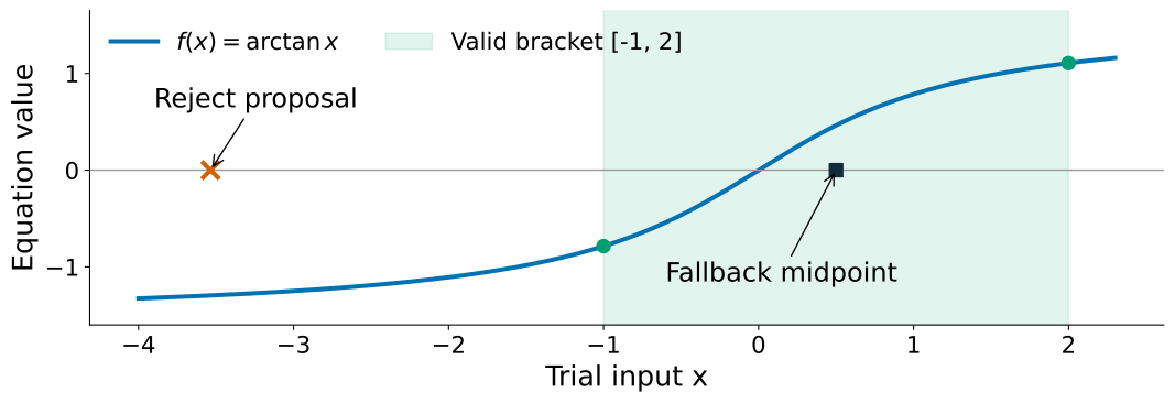
The fallback protects the sign-changing bracket. It does not claim that every accepted local proposal is a root.
Brent’s Method
Combines bisection’s reliability with inverse quadratic interpolation’s speed:
Maintains a bracketing interval like bisection
Tries fast interpolation when possible
Falls back to bisection if interpolation fails
Safeguards maintain convergence from a valid continuous bracket; often needs fewer evaluations than bisection
Practical Strategy for Robust Root Finding
1. Find a continuous sign-change bracket by physics or a scan, then use bisection
2. Propose a local Newton or interpolation step while retaining the bracket
3. Reject unsafe proposals and enforce regular bracket reduction
4. Monitor bracket width, residual scale, stagnation, and evaluation cost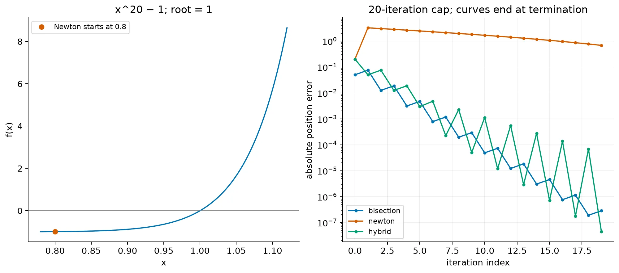
Figure 10:Measured histories for , with root 1. Bisection and the safeguarded Newton method start with ; Newton starts at . All runs have a 20-iteration cap. Bracketed methods stop at half-width 10-10 or a sampled zero. Newton stops at a sampled zero, floating-point stagnation, or the cap. The hybrid takes a midpoint at least every other update. On intervening updates it accepts a finite Newton proposal only strictly inside the bracket; otherwise it also takes the midpoint. This is an illustrative safeguarded Newton method, not Brent’s algorithm. Curves end at termination; zero errors are omitted from the logarithmic axis. A large early Newton step or an unmet iteration cap does not prove eventual divergence. The reference root is exact; this plot reports measured outcomes rather than assigning a universal speed ranking.
All three hard-example runs reach the stated 20-iteration cap. Their final position errors are different; none should be reported as satisfying its stopping contract merely because one plotted error is small.
Investigation: which root estimate is justified?
Suppose three methods report nearly the same root. One stopped because the residual was small, one because the last step was small, and one because a bracket was narrow. These are different observations. Which one controls the position of the root, and what additional information does each require?
Return to the cubic from the opening figure. It is continuous, and on , so a sign-changing bracket there contains one root. Before inspecting the recorded histories, predict:
Must a bisection midpoint become more accurate at every iteration?
Can Newton make a small step without a small position error?
Does one Newton iteration cost the same as one secant iteration?
Which conclusion survives multiplying the whole equation by 10-12?
For this problem, a bracket midpoint has position error at most the half-width. At a candidate in , the derivative bound also gives . The last step is neither of these bounds. It measures what the algorithm just did, not its distance from the answer. Stagnation can make it zero even when a target remains unmet.
The final recorded rows from the cubic comparison are:
| Method | Last recorded step | Actual position error | calls | calls | Stop | |
|---|---|---|---|---|---|---|
| bisection | 6.168e-10 | 5.821e-11 | 5.526e-11 | 36 | 0 | width tolerance |
| newton | 8.882e-16 | 4.441e-16 | 0.000e+00 | 6 | 6 | floating-point stagnation |
| secant | 8.882e-16 | 8.882e-16 | 0.000e+00 | 9 | 0 | floating-point stagnation |
A printed zero position error means agreement with the binary64 reference, not an exact representation of the mathematical root. A sampled zero residual also requires the function-evaluation caveat discussed with bisection.
The comparison figure reports real errors against an independent decimal reference. Those errors are available for this teaching example; the method cannot normally inspect them. Its stopping condition must use information available during the calculation. Count calls to and separately: a derivative may be cheaper, more expensive, or computed together with . An iteration count by itself does not settle the cost comparison.
Explain the evidence before choosing a method
Bisection guarantees that its bound shrinks, not that every midpoint is better than the last. Newton’s last step is a useful diagnostic, but it is not a position certificate. A residual becomes a position bound only with a valid slope bound and reliable function values. Rescaling changes both its residual and derivative scale; the ratio is unchanged when both are scaled consistently. Bracket widths are unchanged too. The physical question and its units determine which reported digits matter.
Transfer: an accurate solve of an uncertain function
Now suppose the function values themselves have a bounded additive uncertainty . This is a different experiment from multiplying an exact equation by a constant. Keep and function values dimensionless, and consider
The unperturbed root is 1. Any perturbed zero obeys . A smaller slope therefore permits a wider range of root positions for the same absolute uncertainty. A tighter iteration tolerance cannot distinguish among those possible input functions.
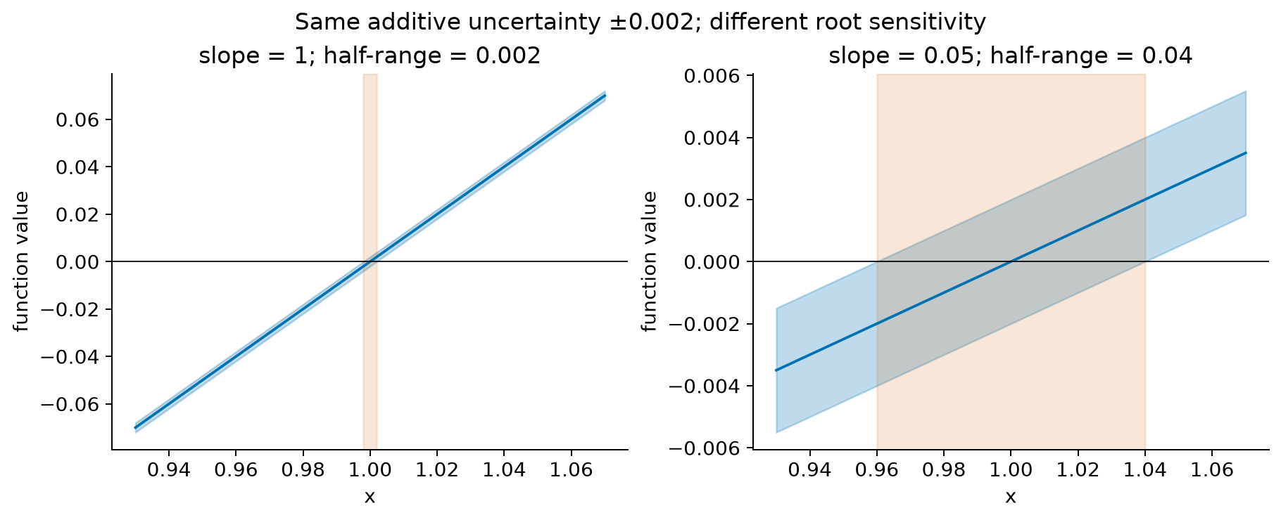
Figure 11:The vertical band represents allowed changes to the supplied function. Its intersection with the horizontal axis gives possible root positions, not iteration histories or statistical confidence intervals. The same uncertainty produces different position ranges because the slopes differ.
# These are possible-input bounds, not errors measured from a root solver.
slopes = np.array([1.0, 0.05])
function_uncertainty = 0.002
root_half_ranges = function_uncertainty / np.abs(slopes)
for slope, half_range in zip(slopes, root_half_ranges):
    print(f"slope={slope:g}: possible roots in [{1-half_range:.3f}, {1+half_range:.3f}]")
slope=1: possible roots in [0.998, 1.002]
slope=0.05: possible roots in [0.960, 1.040]
Predict what happens to this range if we halve the solver tolerance, halve , or multiply both and its uncertainty by 100. Only one of those changes improves the information supplied about the root.
A repeated root makes the issue sharper. For , a downward constant perturbation of size produces two zeros, , while an upward perturbation removes the real zero. There is no nonzero derivative lower bound at the original root. For the unperturbed function, Newton’s exact recurrence is
A tiny residual is especially easy to obtain here because it is the square of the position error. For example, residual 10-12 corresponds to position error 10-6, not 10-12.
Answer: what would justify another digit?
Halving the solver tolerance only refines a solve of the supplied function. Halving the input uncertainty narrows the possible-root interval. Multiplying both the function and its uncertainty by 100 leaves the interval unchanged. For a repeated root, a smooth-simple-root theorem cannot justify quadratic convergence or convert the residual through a nonzero slope bound. Before reporting more digits, distinguish iteration error from uncertainty in the function being solved; then identify which independent calculation or better measurement would reduce the limiting contribution.
Further reading: conditioning, residuals, and multiple roots.
Application: Units and Scaling
Choose scales that make the variables and tolerances interpretable. Non-dimensionalization can avoid extreme arithmetic and improve numerical balancing, but it does not remove intrinsic sensitivity:
Dimensional form: Finding radius where g/cm with in cm Scaled form: Define , and solve (equal to 1 only if that target is the chosen )
Track the units of the position tolerance and transform it with the variable. Rescaling an equation changes its residual values; it does not by itself make a root better determined by the physical data.
Physical Example: Stellar Structure Equilibrium
In stellar interiors, hydrostatic equilibrium requires:
For a polytrope with , the Lane-Emden equation describes stellar structure:
where is dimensionless radius and is related to density.
The stellar surface occurs where —a root-finding problem!
For different polytropic indices:
is the constant-density Lane–Emden limit: , so .
has , with its central value defined by the limit 1; . This is a polytrope, not an isothermal core.
has and appears in idealized radiation-supported and relativistically degenerate models.
has : it approaches zero only at infinite radius, although its total mass is finite. It is not a minimum-mass-star model.
These solutions use and . Reference: analytic polytropes.
A computed Lane–Emden trajectory can supply both and its derivative near the surface. Root refinement then depends on the accuracy of that trajectory as well as on the root solver. Tightening a root tolerance cannot remove the ODE or interpolation error. Preserve a credible surface bracket and refine the underlying trajectory before claiming additional digits.
Worked Example: Kepler’s Equation
The most famous root-finding problem in astronomy is Kepler’s equation, which relates mean anomaly (proportional to time) to eccentric anomaly (related to position):
where is the orbital eccentricity and both and are in radians.
Why This Is Hard
Transcendental equation (no algebraic solution)
Must be solved millions of times in orbit propagation
High eccentricity makes convergence difficult
Conditioning worsens as (parabolic orbit)
Newton’s Method Applied
Define
Then
Newton iteration:
For an ellipse, , so . The derivative can become small near periapsis as approaches 1, but it cannot vanish in this domain.
Initial Guess Strategy
One heuristic on a reduced mean-anomaly interval is to start with for and otherwise. The value 0.8 is not a convergence threshold, and the first regime is not uniformly nearly circular. Compare both guesses over the project’s sweep and report failures and iteration counts. If reducing modulo , restore its branch in the returned .
Convergence Analysis
The absolute sensitivity to mean anomaly is
For , exactly. For the upper bound is 10, and for it is 100; these are bounds, not the sensitivity at every orbital phase. Iteration counts also depend on , the initial guess, and the stopping criterion. Normalize to for the initial-guess choices above. Because the residual is increasing and changes sign on for an interior , bisection provides a useful independent check on Newton’s answer.
Practical Algorithm for Finding Initial Brackets
To find initial brackets for bisection:
def find_brackets(f, x_min, x_max, n_scan=100):
    """Return sign-change intervals and (x, x) pairs for sampled zeros."""
    if isinstance(n_scan, (bool, np.bool_)) or not isinstance(n_scan, (int, np.integer)) or n_scan <= 0:
        raise ValueError("n_scan must be a positive integer")
    if not (np.isfinite(x_min) and np.isfinite(x_max) and x_min < x_max):
        raise ValueError("Need finite increasing scan limits")
    nodes = np.linspace(x_min, x_max, n_scan + 1)
    values = np.array([float(f(x)) for x in nodes])
    if not np.all(np.isfinite(values)):
        raise ValueError("Non-finite value in scan")
    brackets = []
    for i, (x, fx) in enumerate(zip(nodes, values)):
        if fx == 0.0:
            brackets.append((x, x))
        elif i > 0 and values[i-1] != 0.0 and (values[i-1] < 0) != (fx < 0):
            brackets.append((nodes[i-1], x))
    return brackets

print(find_brackets(lambda x: x - 0.5, 0.0, 1.0))
[(np.float64(0.5), np.float64(0.5))]
A scan can miss an even-multiplicity root between samples or several crossings
within one cell. A sampled zero is reported once, as a zero-width pair; the
reading’s bisection accepts it. Project 3’s bisect requires a < b,
so retain these sampled roots separately and send only positive-width brackets
to that solver. Neither a sign scan nor bisection proves
continuity or verifies that a computed zero did not arise from underflow.
Debugging Root Finding
Common root-finding bugs and their diagnosis:
| Symptom | Likely Cause | Fix |
|---|---|---|
| Bisection won’t start | Same sign at endpoints | Scan for sign changes first |
| Newton diverges | Poor initial guess or a small derivative | Find and verify a sign-changing bracket first, then apply bisection; a line search is another step-control option with different guarantees |
| Secant oscillates | An unreliable slope or poor starting points | Inspect the function-value scale, separation of inputs, and proposed step; reject zero/nonfinite denominators or unusable updates, then restart or safeguard |
| Wrong root found | Multiple roots in region | Narrow search interval |
| No progress | No representable interior point or unmet iteration cap | Report failure; reassess position tolerance and scaling |
| No convergence | Discontinuous function | Check function continuity |
Bridge to Part 2: From Finding Zeros to Measuring Areas
You can now compare three kinds of evidence: a shrinking bracket, a local iteration model, and a residual interpreted through sensitivity. A method choice should identify which of these supports the reported root.
But finding equilibrium points is only half the story. Next, we tackle integration — measuring quantities across space and time. You’ll discover how the same principles of approximation and error analysis apply to computing areas under curves, volumes of regions, and integrals over high-dimensional spaces.
The synthesis returns to a problem in which an integral defines the root residual. The two algorithms have separate jobs, but their errors contribute to one final answer.
Next: Part 2 - Quadrature