Part 2: Quadrature — Discrete Sums, Error, and Adaptation
Module 2: Static Problems & Quadrature | COMP 521
Learning Objectives
By the end of this section, you will be able to:
Derive rectangular, trapezoidal, and Simpson’s rules from Taylor series
Understand optimal point placement through Gaussian quadrature basics
Implement a quadrature rule as a reusable function of a callable, interval, and panel count, then test its contract with
pytest.Explain adaptive refinement, a change of variables at a branch point, and Monte Carlo’s root-mean-square error model.
Choose an appropriate method from smoothness, sampling access, dimension, and a measured error regime rather than a fixed dimension cutoff.
Analyze error scaling and predict convergence behavior before floating-point round-off dominates.
Building a reusable numerical method
Project 2 is the first course project in which reusable code belongs in Python modules rather than only in a notebook. The central interface is
rule(f, a, b, n)where f is a callable that accepts a NumPy array of sample positions and
returns matching numeric values; a and b are integration limits; and n is
the positive integer number of subintervals. The algorithm must not know whether
f represents a sine wave, a Planck spectrum, or a limb-darkened stellar disk.
Put the rules in integrate.py, write the figures and interpretation in
analysis.ipynb, and run python -m pytest from the project root. A test makes
one part of the contract visible: a known integral, an exactness property, an
invalid panel count, or a predicted convergence ratio. The course
software engineering guide
and workflow checklist
give the corresponding repository workflow.
Do not introduce a class for these rules. A rule has no persistent state: every
call receives its callable, interval, and panel count. Project 3 introduces
classes when a Star owns related state and invariants that must remain
consistent.
The Fundamental Challenge
While differentiation is a local operation (needing only nearby points), integration is global — we must consider the entire domain. Quadrature (numerical integration) transforms the continuous integral:
into a discrete sum:
The numerical question is not only how to choose:
The points (where to sample)
The weights (how much each sample contributes)
The number (balancing accuracy vs computation)
It is also how to state and test the rule’s inputs, preconditions, and expected error. A correct answer for one integrand does not establish a reusable method.
Physical Motivation: Why Astronomers Integrate
Integration is everywhere in astronomy because we observe integrated quantities:
Spectroscopy: A finite wavelength band collects integrated spectral flux
Photometry: CCD pixels integrate photons over exposure time
Structure: Mass distributions require volume integrals
Cosmology: In a spatially flat cosmology, luminosity distance involves integrating through expanding space
Each context demands different accuracy, and the function properties (smooth vs oscillatory, bounded vs singular) determine the best method.
Resolution is not conditioning: An oscillatory or rapidly varying integrand may need many samples to resolve. That is not, by itself, a statement that the integral is ill-conditioned; conditioning asks how strongly the exact integral changes when the input function is perturbed.
Building Integration Methods: From Rectangles to Optimality
The Riemann Sum Foundation
The definition of the Riemann integral suggests the simplest approximation:
where and .
Different choices of give different methods:
Left endpoint: Rectangle rule (left)
Right endpoint: Rectangle rule (right)
Midpoint: Midpoint rule
Average of endpoint heights: Trapezoidal rule (an average of two samples, rather than one Riemann sample)
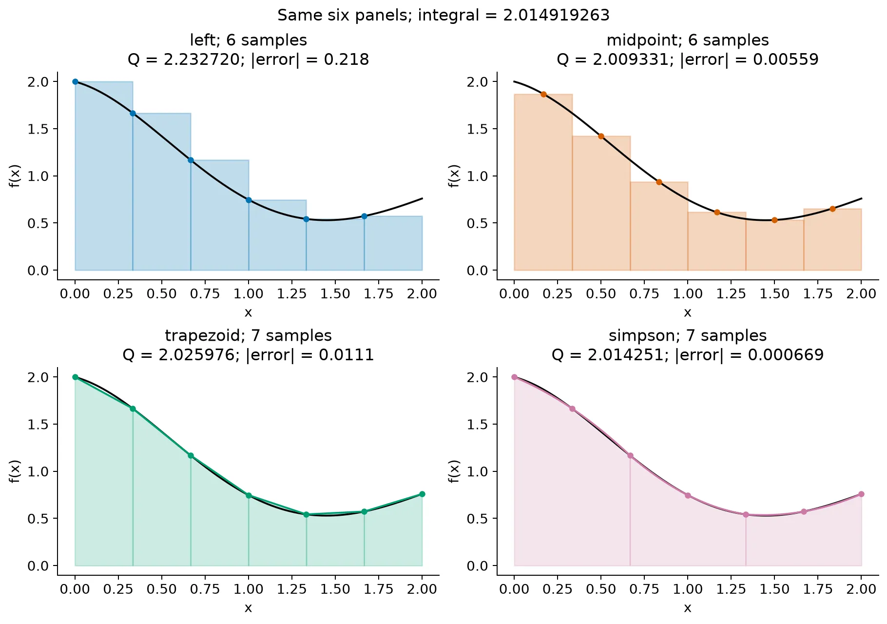
Figure 1:Four quadrature approximations to the dimensionless integral of from 0 to 2, all with six panels. Left and midpoint rules use six sample values; trapezoid and Simpson use seven. Colored areas show the actual constant, linear, or quadratic interpolants used by the rule. The black curve is the integrand. Reported errors use its analytic antiderivative as a common reference.
Method 1: Left Rectangle Rule
Purpose: This baseline rule makes the local-to-global error calculation visible.
Mathematical Formulation
For uniform spacing :
Error Analysis via Taylor Series
On each subinterval :
Evaluating:
The rectangle rule uses only , so the signed local error is
Over intervals:
First-order method: Global error proportional to step size.
This is a first-order method: in the truncation-dominated regime, halving halves the leading global error.
Turn a slope bound into a panel count
Suppose , is continuously differentiable, and on . Within a panel, the mean value theorem gives . Integrating the height discrepancy gives
Geometrically, this is a triangle of base and maximum height . Summing the absolute panel bounds and using yields
For a target absolute quadrature error , a sufficient integer count is . A bound may be conservative: it permits the largest slope on every panel and ignores cancellation. A maximum observed on a sampled plot is not automatically a rigorous derivative bound.
For sine on , and , so the bound is . At it is below 0.01, which justifies the accuracy scale in the module test below. This bound concerns quadrature in exact arithmetic; check that floating-point effects are small compared with the test margin.
Move the sample, keep the panels
Right rectangles use ; midpoint rectangles use . For increasing functions the left sum is below the integral and the right sum is above it. Their difference telescopes to . Midpoint symmetry cancels the first-derivative contribution, giving composite error when the second derivative is bounded. Averaging the left and right sums gives the trapezoid rule, which we derive next.
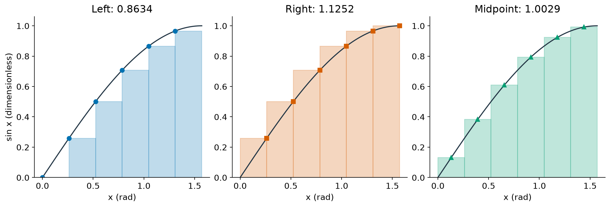
For sine on , left rectangles underestimate and right rectangles overestimate. Midpoint rectangles slightly overestimate because the curve is concave down; they do not have the same first-order bias as endpoint rectangles.
Implementation
import numpy as np


def rectangle(f, a: float, b: float, n: int) -> float:
    """Approximate an integral with the left rectangle rule (global order 1)."""
    if isinstance(n, bool) or not isinstance(n, (int, np.integer)) or n <= 0:
        raise ValueError("n must be a positive integer.")

    a_float = float(a)
    b_float = float(b)
    if not (np.isfinite(a_float) and np.isfinite(b_float)):
        raise ValueError("a and b must be finite.")

    h = (b_float - a_float) / n
    x = a_float + h * np.arange(n)
    values = np.asarray(f(x), dtype=float)
    if values.shape != x.shape:
        raise ValueError("f must return one numeric value for each sample position.")
    if not np.all(np.isfinite(values)):
        raise ValueError("f returned a non-finite sample value.")
    return float(h * np.sum(values))


exact_sine_integral = 1.0
for panel_count in (8, 16, 32):
    approximation = rectangle(np.sin, 0.0, np.pi / 2.0, panel_count)
    absolute_error = abs(approximation - exact_sine_integral)
    print(
        f"n = {panel_count:2d}; "
        f"left rectangle = {approximation:.10f}; "
        f"absolute error = {absolute_error:.3e}"
    )
n = 8; left rectangle = 0.8986104015; absolute error = 1.014e-01
n = 16; left rectangle = 0.9501092953; absolute error = 4.989e-02
n = 32; left rectangle = 0.9752555017; absolute error = 2.474e-02
What the rectangle rule can and cannot establish
Its global error is only first order for smooth functions.
For a monotonic function it has a one-sided bias: it underestimates an increasing function and overestimates a decreasing function when .
It is a useful baseline in Project 2 because its measured order of 1 makes the improvement to orders 2 and 4 visible.
It is not automatically the right choice when higher accuracy per function evaluation is needed.
First tests for a module
Put the implementation in integrate.py and a separate test file in tests/.
The test below checks a known integral and one invalid input. It checks the
public behavior, not the rule’s internal loop or array construction.
# tests/test_integrate.py
import numpy as np
import pytest

from integrate import rectangle


def test_left_rectangle_sine_is_a_lower_estimate() -> None:
    approximation = rectangle(np.sin, 0.0, np.pi / 2.0, 128)
    assert approximation < 1.0
    assert 1.0 - approximation < 0.01


def test_rectangle_rejects_nonpositive_panel_count() -> None:
    with pytest.raises(ValueError):
        rectangle(np.sin, 0.0, np.pi / 2.0, 0)
Add comparable tests for trapezoid and simpson: an exactly integrated
polynomial where appropriate, a convergence comparison on a smooth function,
and each rule’s invalid-input behavior. The test tolerance must follow a stated
error scale, not an arbitrary number of decimal places.
Method 2: Trapezoidal Rule
Why we care: The trapezoid rule is a clear second-order rule for a smooth callable and a natural rule for already tabulated data.
Geometric Intuition
Instead of rectangles, connect consecutive points with straight lines, creating trapezoids. The area of each trapezoid averages the function values at its endpoints.
Mathematical Formulation
The area of a trapezoid with parallel sides and and height is:
Summing over all intervals:
Error Analysis
Using Taylor expansion around the midpoint :
The trapezoidal approximation on :
Put and integrate the same Taylor polynomial from to . The odd term vanishes:
Subtracting the trapezoid gives at leading order. With continuous , the exact remainder can be expressed at some point in the panel:
Local error:
Second-order method: Global error is proportional to step size squared.
Global error: for some
This is a second-order method: doubling the number of panels reduces the leading error by about a factor of 4 while the asymptotic model holds.
Common Failure Modes and Fixes
| Problem | Symptom | Solution |
|---|---|---|
| Endpoint singularity | Non-finite sample or order loss | Use a limiting value, a justified cutoff, or a change of variables |
| Oscillations | Poor convergence | Resolve the oscillation, split the domain, or use a method designed for it |
| Noisy sampled data | A noisy integral estimate | Report data uncertainty; smoothing is a modeling decision, not an automatic numerical fix |
| Discontinuity or kink | Error changes; a derivative kink can retain order 2, while a jump can reduce it | Split at the known feature and measure the resulting convergence |
Method 3: Composite Simpson’s Rule
Why we care: For a sufficiently smooth integrand, Simpson’s symmetric two-panel construction gives fourth-order global error.
The Key Insight
Instead of linear interpolation (trapezoids), use quadratic interpolation (parabolas) through consecutive triplets of points.
Derivation via Interpolation
For three equally-spaced points with and , the unique parabola through is:
Integrating this parabola from to :
These are the famous Simpson weights: 1, 4, 1.
Composite Simpson’s Rule
For intervals (must be even):
The pattern of weights is:
Endpoints: 1
Odd indices (1,3,5,...,n-1): 4
Even indices (2,4,6,...,n-2): 2
Error Analysis and Fourth-Order Accuracy
Through careful Taylor series analysis, the local error for Simpson’s rule on interval is:
Fourth-order method: The leading global truncation error is proportional to when the smoothness assumptions hold.
Global error:
Simpson’s rule is fourth-order accurate under these assumptions.
Why Simpson’s Rule is Fourth-Order
Expand about the fixed midpoint , writing with . For with a continuous fourth derivative, Taylor’s theorem gives
Both the exact integral and Simpson’s symmetric weighted sum cancel the odd terms. In particular, is one fixed coefficient, so
Simpson’s rule also integrates the constant and quadratic terms exactly. The remaining contribution gives error over this panel pair; summing pairs gives composite error. This establishes the order; the error formula above supplies its coefficient and sign. For a cubic polynomial the remainder is zero, so Simpson is exact in exact arithmetic.
The interpolation remainder instead contains , whose evaluation point can vary with . We cannot assume that entire remainder is odd. The fixed-midpoint Taylor expansion is what justifies the cancellation.
Recover the error coefficient, not only the order
For a sufficiently smooth function, the quartic Taylor term at midpoint is . Over , its exact integral is
Simpson’s weighted sum of that term is
Subtracting gives at leading order. There are panel pairs, which explains the composite coefficient . This Taylor calculation explains the coefficient; the exact remainder theorem with continuous fourth derivative places its evaluation at an appropriate rather than necessarily at the midpoint.
For on , the difference is exactly : makes the same prediction. This is a useful sign and coefficient check, distinct from checking exactness on cubics.
When Simpson’s Rule Shines
Smooth functions with continuous fourth derivative
Smooth functions without exploitable periodic endpoint matching; see the periodic comparison below
When high accuracy is needed with moderate
Physical models whose regularity has been checked, including at boundaries
Common Failure Modes and Fixes
| Problem | Symptom | Solution |
|---|---|---|
Odd n | The panel pairing is undefined | Raise ValueError; Project 2 requires an even panel count |
| Noisy sampled data | Higher order does not remove uncertainty | Use an uncertainty model; choose a rule appropriate to the samples |
| Insufficient regularity for the quoted remainder theorem | Its theorem no longer certifies the order | Inspect the actual feature and measure convergence; discontinuity of alone does not force order loss |
| Sharp local features | Fixed panels miss the feature | Refine locally or use adaptive quadrature |
Answers and reasoning
Each quadratic interpolant spans two subintervals, so composite Simpson pairs an even number of subintervals.
Simpson integrates a cubic exactly in exact arithmetic: the symmetric odd remainder cancels, even though the interpolant is quadratic. Floating-point evaluation can still leave a small discrepancy.
Doubling halves and reduces a nonzero dominant fourth-order error by approximately 16. This prediction fails outside the smooth, resolved truncation regime.
Discontinuities, endpoint singularities, unresolved oscillations, or noisy data can violate that regime. Inspect the integrand and refine; the method name is not evidence that the assumptions hold.
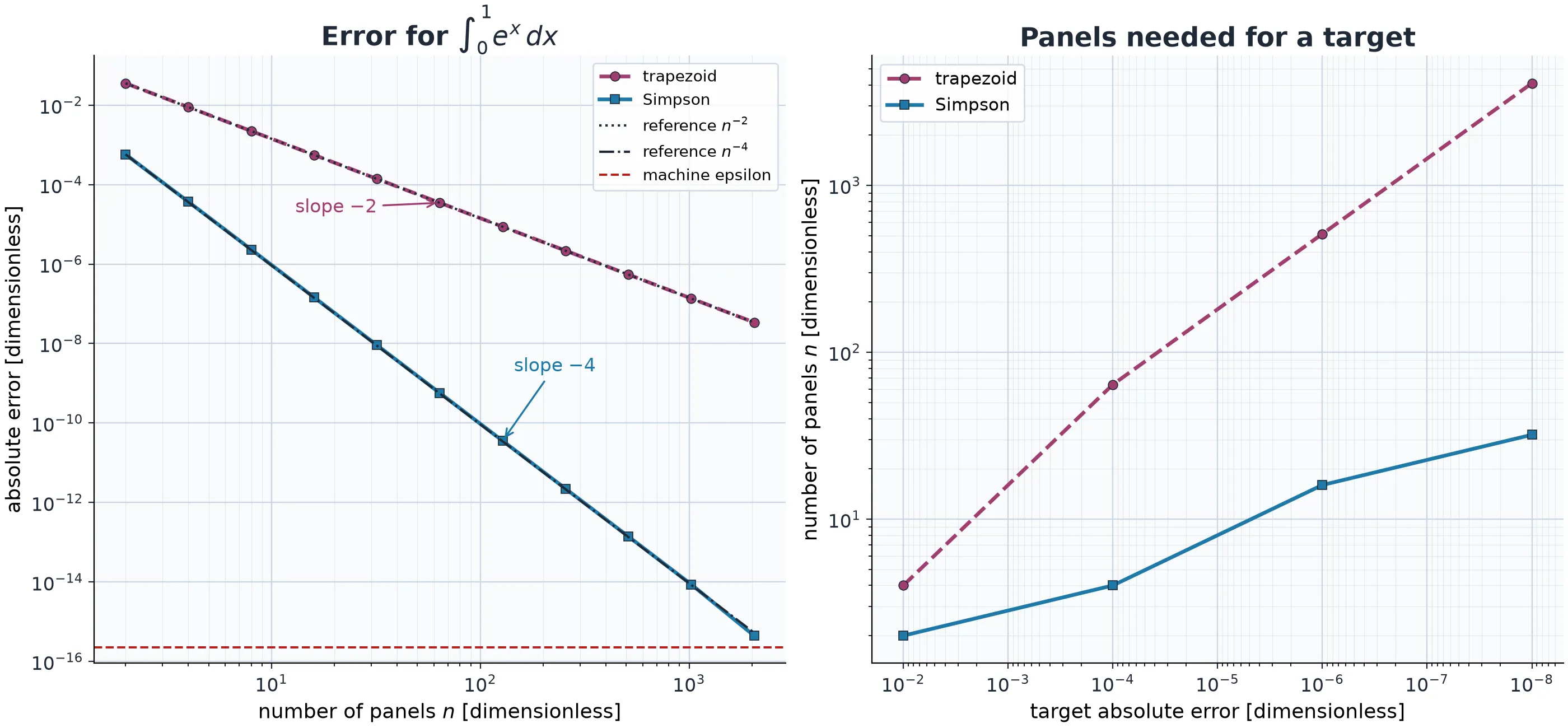
Figure 3:Error scaling for the dimensionless integral . The left log-log panel plots absolute error against the number of panels ; the trapezoid and Simpson trends have slopes -2 and -4 before the floating-point floor. The right panel compares the panel counts required for stated absolute-error targets. Circle and square markers, and dashed and solid lines, distinguish the rules as well as color.
Extension: periodic endpoints can change the comparison
The second-order trapezoid formula is a general smooth-function result, not an upper limit on what a particular problem can achieve. For smooth periodic functions integrated over a complete period, matching endpoint derivatives can cancel successive error terms. Analytic periodic functions can exhibit exponential convergence with the number of equally spaced samples. Further reading: spectrally accurate integration.
For a controlled dimensionless example, take and
Its integral on is . The periodic trapezoid sum averages all nonaliased cosine modes to zero, leaving an exact-arithmetic error
For , the reference comparison below uses the same uniform samples for trapezoid and Simpson. Neither method receives an advantage in sample count. Do not interpret a result near floating-point precision as an indefinitely continuing exponential trend.
| Panels | Trapezoid absolute error | Simpson absolute error |
|---|---|---|
| 4 | 8.378e-01 | 2.793e-01 |
| 8 | 4.928e-02 | 2.135e-01 |
| 16 | 1.918e-04 | 1.617e-02 |
| 32 | 2.926e-09 | 6.391e-05 |
Simpson combines nested trapezoid estimates as . Here the coarser trapezoid contribution can dominate its error: cancelling an term is unhelpful when that term was already absent. The lesson is to inspect the problem’s structure and measured cost, not to replace one universal method ranking with another.
Method 4: Gaussian Quadrature
Why we care: When samples can be chosen, their placement and weights can carry more information than a uniform grid with the same number of evaluations.
The main idea
The previous composite rules used equally spaced points. Gaussian rules instead choose both nodes and weights for a specified weight function.
For points, Gauss--Legendre quadrature is exact for every polynomial up to
degree when it uses the roots of the Legendre polynomial of degree
and their associated weights. This exactness statement is more precise than an
O(h^p) order claim: a fixed -point rule has no grid spacing .
Example: 2-Point Gaussian Quadrature
Instead of evaluating at equally-spaced points, Gaussian quadrature uses special points. For 2 points on :
Points: ,
Weights:
This choice makes the rule exact for all cubic polynomials.
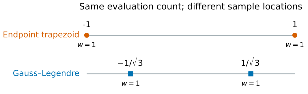
Both rules evaluate twice. Their sample locations differ, and the Gaussian weights apply to function values rather than to fixed-width panels.
For , the endpoint trapezoid gives 2, while these Gaussian nodes give , the exact integral on .
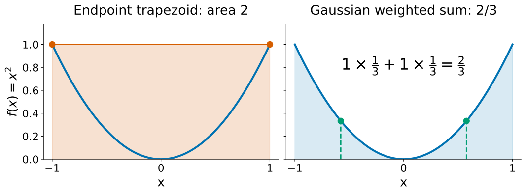
The right-hand shading is the true integral, not a collection of Gaussian panels. Gaussian quadrature combines the two sampled values with their weights.
In Practice
NumPy provides the nodes and weights. This is an extension, not a Project 2 implementation target.
from numpy.polynomial.legendre import leggauss


def gauss_legendre(f, a: float, b: float, n: int) -> float:
    """Apply an n-point Gauss--Legendre rule on [a, b]."""
    if isinstance(n, bool) or not isinstance(n, (int, np.integer)) or n <= 0:
        raise ValueError("n must be a positive integer.")
    points, weights = leggauss(n)
    x_gauss = (b - a) * points / 2.0 + (a + b) / 2.0
    return float((b - a) * np.sum(weights * f(x_gauss)) / 2.0)


print(f"2-point rule on x**3 over [0, 1]: {gauss_legendre(lambda x: x**3, 0.0, 1.0, 2):.16f}")
2-point rule on x**3 over [0, 1]: 0.2500000000000000
When Gaussian Quadrature Matters
When you control where to sample (not experimental data)
For very smooth functions
When function evaluations are expensive (fewer points needed)
As the foundation for spectral methods in advanced simulations
The general lesson is that sample placement is part of a numerical method, not a detail to leave implicit.
Method 5: Monte Carlo Integration
Why we care: Monte Carlo replaces a grid by a random average. Its root-mean-square rate does not explicitly depend on dimension, but its usefulness still depends on the integrand variance and sampling strategy.
Understanding Dimensions in Integration
Integration dimension: The number of independent variables being integrated over. A triple integral f(x,y,z) dxdydz is 3-dimensional, not because it’s in 3D space, but because we integrate over 3 variables.
When we talk about “dimensions” in Monte Carlo integration, we mean the number of integration variables, not spatial dimensions:
1D integral: (one integration variable)
2D integral: (two integration variables)
6N-D integral: Phase space integral over N particles with 3 position and 3 momentum components each
For example, a classical configurational partition function for 100 atoms has 300 position coordinates. The full phase-space formulation also includes momenta; for a separable quadratic kinetic energy, those momentum integrals can be done analytically.
The Curse of Dimensionality
Curse of dimensionality: Exponential growth of computational cost with dimension for grid-based methods.
For a -dimensional integral with points per dimension, a full tensor-product grid needs evaluations:
1D: 100 points
2D: 1002 = 10,000 points
3D: 1003 = 1,000,000 points
10D: 10010 = 1020 points (impossible!)
This exponential growth is why tensor-product grids become expensive quickly. It does not establish one dimension at which every deterministic method fails or Monte Carlo becomes best: smoothness, structure, error target, and available variance reduction all matter.
The Monte Carlo Solution
Draw independent, identically distributed points uniformly from a domain with finite, nonzero volume:
where is the volume of the domain. Uniform sampling is essential to this formula. Sampling from a nonuniform density instead requires importance weights , with wherever the integrand contributes.
Error Analysis
Central Limit Theorem: For independent, identically distributed samples with finite variance, the centered and appropriately scaled sample mean approaches a normal distribution.
For the Monte Carlo estimator :
Step 1: The expected value of our estimator is the true integral:
Step 2: The variance of the estimator is:
where is the finite variance of under uniform sampling over the domain.
Step 3: The standard error (standard deviation of the estimator) is:
Dimension-independent convergence: Monte Carlo error scales as regardless of dimension d!
Key insight: Error independent of dimension !
This model assumes:
Independent random samples
Finite variance of the integrand ()
A sample size large enough that the observed estimator distribution is in the regime being summarized; there is no universal cutoff such as
The rate says nothing about the constant . A high-variance integrand can have a large error even when the slope is correct.
Choosing Monte Carlo honestly
In one dimension, the deterministic rules in this project usually beat plain Monte Carlo on smooth integrands. Monte Carlo becomes attractive when a useful deterministic grid would require many samples across many integration variables, or when a sampling distribution can reduce variance. Compare methods at a stated evaluation budget; do not choose from a dimension cutoff alone.
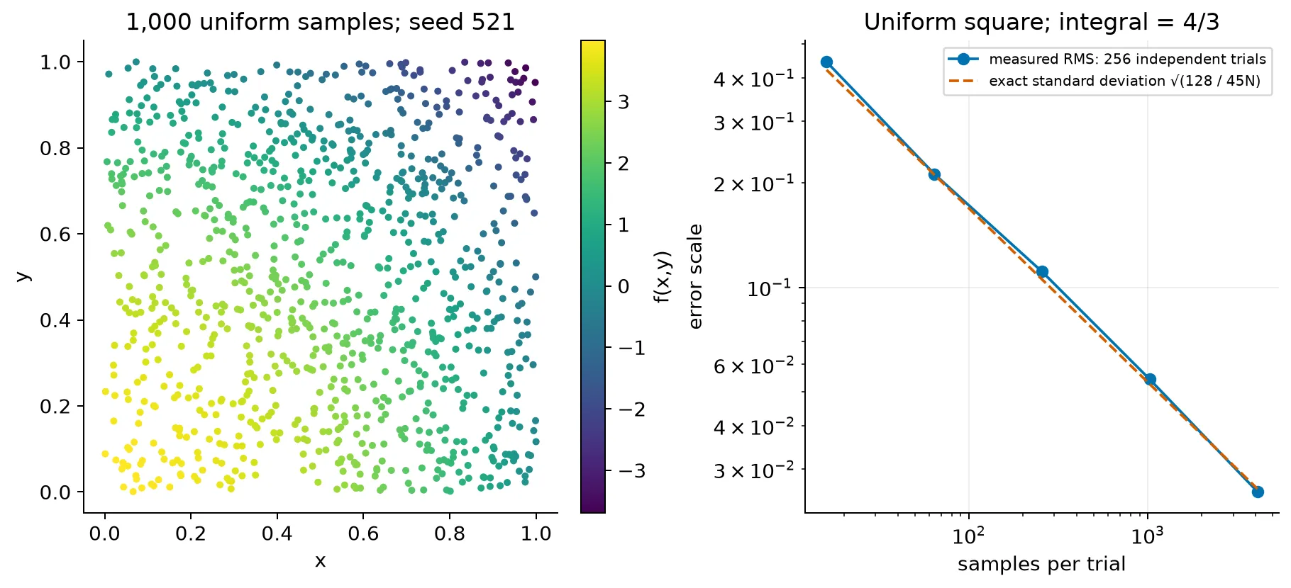
Figure 6:Monte Carlo integration. The left panel shows random samples of a two-dimensional integrand over a square domain; their average, multiplied by the domain area, estimates the integral. The right log-log panel reports RMS error from 256 independent trials at each sample count, with reproducible seed 521. For this integrand, the variance under uniform sampling is , so the estimator standard deviation is . The theoretical curve has slope ; measured RMS fluctuates around it. This statement requires independent finite-variance sampling and does not describe every individual error.
Common Failure Modes and Fixes
| Problem | Symptom | Solution |
|---|---|---|
| Infinite variance | The usual standard-error model fails | Change variables or construct an estimator with finite variance |
| Rare events | High-variance estimate | Use importance or stratified sampling with a justified proposal |
| Correlated samples | Fewer effective samples than | Diagnose autocorrelation and report effective sample size when applicable |
| One run happens to be close | An uninformative small signed error | Use independent seeded trials and summarize RMS error or a standard error |
Adaptive Methods and Richardson Extrapolation
Adaptive Quadrature
Adaptive quadrature changes the number and location of panels rather than using one fixed spacing everywhere. For composite Simpson’s rule, compare one Simpson estimate on , , with the sum of two Simpson estimates on its halves, . Since Simpson’s leading global error is proportional to ,
Under the leading-error model, the finer-grid estimate uses the factor . Comparing the two approximations
directly to tol uses the wrong scale and rejects intervals more often than the
stated tolerance requires.
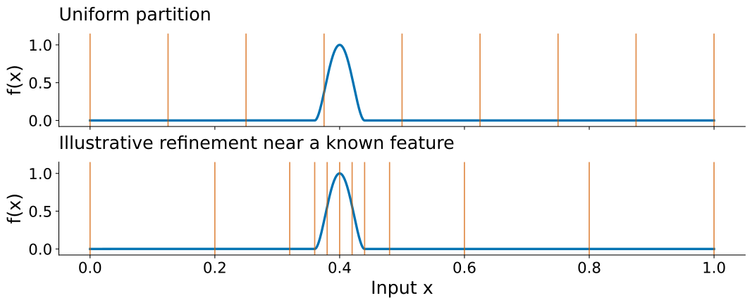
Local refinement spends more samples near a feature. This illustrative partition uses its known location; it is not an adaptive solver trace.
For Project 2, the public interface is
adaptive_simpson(f, a, b, tol, max_depth=50)The algorithm is recursive but its contract is ordinary and testable:
Validate that
tolis positive and thatmax_depthis a non-negative integer; otherwise raiseValueError.Compute , , and from their shared endpoint and midpoint values.
If the error estimate meets the local tolerance, return the corrected estimate .
Otherwise, if no recursion depth remains, raise
RuntimeError; a partial integral is not a valid answer.Recurse on the two halves with
tol / 2for each, then add their estimates.
Halving the tolerance is a simple equal allocation: the two child error budgets add to the
parent budget. A max_depth guard is equally necessary because a singularity,
non-finite value, or unrealistically small tolerance can otherwise recurse until
Python fails without explaining the numerical problem.
Adaptive subdivision is not root finding. It bisects intervals to control an integral-error estimate; it does not require a sign-changing bracket or select a solution of . Root-finding methods and their contracts begin in Block 3.
Absolute and relative error budgets
The Project 2 tol is an absolute integral-error budget, in units of
. It is not the root-position tolerance used by a root finder.
A more general integrator can compare an estimated error with
where estimates the integral, carries the integral’s units, and is dimensionless. This explains a common library interface; it does not change Project 2’s required signature.
If positive and negative contributions nearly cancel, may be tiny even when is large. A purely relative target based on can then be unrealistic. Choose an absolute scale from the question and the uncertainty in the supplied function; do not promise relative digits that cancellation and round-off cannot support.
Local budgets must also support the global claim. The Project 2 allocation
tol/2 makes child absolute budgets sum to their parent’s budget. Giving every
subinterval the full tolerance does not preserve that bound. Separately
accepting relative errors against each subintegral can likewise overstate
accuracy in a strongly cancelling sum. A general absolute/relative controller
needs to account for accumulated error estimates and the total-result scale.
The estimate assumes a resolved smooth-error regime. It estimates the error of the finer Simpson value; applying the correction does not turn the estimate into a rigorous error bound for every integrand. Check refinement, known breakpoints, analytic cases, and recursion failures. The missed-feature example below shows why tightening a tolerance alone may not help.
See FNC’s adaptive integration chapter for the connection between extrapolation, error estimation, cancellation, and mixed absolute/relative criteria.
Predict → Run → Explain: an adaptive estimate can miss structure
Error estimation compares what was sampled. It cannot see an oscillation whose zeros coincide with all of its first sample positions. Consider on . Its exact integral is . Predict the initial Simpson estimates at .
def simpson_panel(f, a, b):
    midpoint = (a + b) / 2
    return (b-a) * (f(a) + 4*f(midpoint) + f(b)) / 6

hidden_wave = lambda x: np.sin(4*np.pi*x)**2
whole = simpson_panel(hidden_wave, 0.0, 1.0)
two = simpson_panel(hidden_wave, 0.0, 0.5) + simpson_panel(hidden_wave, 0.5, 1.0)
estimated_error = abs(two-whole) / 15
corrected = two + (two-whole) / 15
print("estimated error:", estimated_error)
print("actual error:", abs(corrected - 0.5))
print("values between original samples:", hidden_wave(np.array([0.125, 0.375])))
estimated error: 7.298429501691755e-49
actual error: 0.5
values between original samples: [1. 1.]
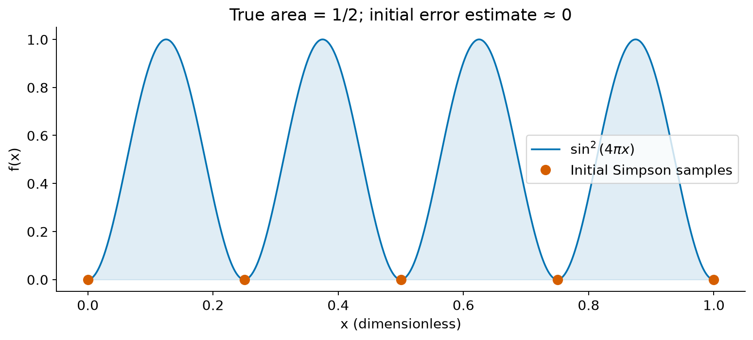
The initial sample values are nearly zero in floating point, while the curve has substantial area between them. Agreement between two unresolved estimates does not establish an accurate integral.
The estimate is effectively zero, yet the corrected answer misses about 0.5. The leading-error model has not been reached. Known oscillation scales, domain splitting, minimum resolution, shifted diagnostic samples, and independent refinement can reveal this failure. No finite collection of samples can guarantee an integral for every unrestricted continuous function. A theorem needs additional information, such as derivative bounds or known structure.
Answer: what would a smaller tolerance change?
An ordinary tolerance smaller than 10-8 can still accept this initial estimate: both sampled approximations are near zero. More stringent acceptance of the same misleading estimate is not the repair. Sampling between the old nodes reveals the peaks; then refine enough to measure the expected regime. The stopping rule controls an estimate, not an unconditional true-error bound.
Now change the sampling rather than the acceptance threshold. A separate fixed-grid reference calculation for this same wave gives:
| Composite Simpson panels | Distinct sample positions | Integral estimate |
|---|---|---|
| 4 | 5 | approximately 0 |
| 8 | 9 | approximately |
| 16 | 17 | approximately |
| 32 | 33 | approximately |
The first refinement reveals the missed area but overestimates it. The next resolves enough of this particular trigonometric function to obtain its exact integral up to rounding. This is evidence about the stated wave and grids, not a universal minimum panel count. The check changes what the algorithm can observe; shrinking a tolerance applied to the original samples does not.
Richardson Extrapolation
Richardson Extrapolation: Using results at different resolutions to cancel leading error terms and achieve higher accuracy.
If your method has error , compute at two resolutions:
This cancels the leading error term! For trapezoidal rule (p=2):
For a sufficiently smooth integrand on nested uniform grids, the trapezoid error expansion has even powers: after cancelling the term, the next term is . The general expansion written above alone would promise only ; the extra order comes from symmetry.
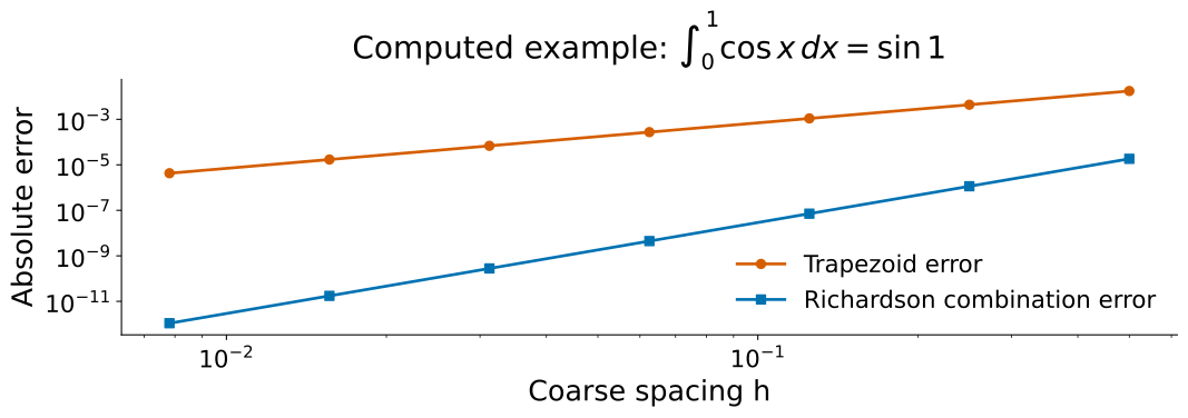
For this smooth, resolved cosine example, the measured combination follows a steeper error trend. The plot is evidence for this example, not a universal error guarantee.
Investigation: why did the expected order disappear?
A correct implementation can fail to show its nominal order on a particular integrand. To tell a bug from a violated assumption, keep the rule fixed and change one feature of the problem. We will use composite Simpson and return to the smooth reference .
Predict: connect the shape to the error model
Compare two dimensionless integrands on :
The second has a kink at . Its integral is also known:
Before inspecting the figure, predict which of these statements is justified:
Halving the panel width should reduce a nonzero leading Simpson error by 16 on a sufficiently smooth, resolved problem.
The same factor must hold for because its function values are finite.
Splitting at the kink makes each piece smooth, allowing the fourth-order model to be tested separately on the two pieces.
The location never lies on these dyadic unsplit grids. This avoids hiding the feature accidentally at a node. The split calculation uses half of the panels on each side and reuses the common endpoint. Both calculations therefore have the same total panel count and distinct function samples; their local widths differ. The comparison asks what sample placement and regularity change at equal evaluation count.
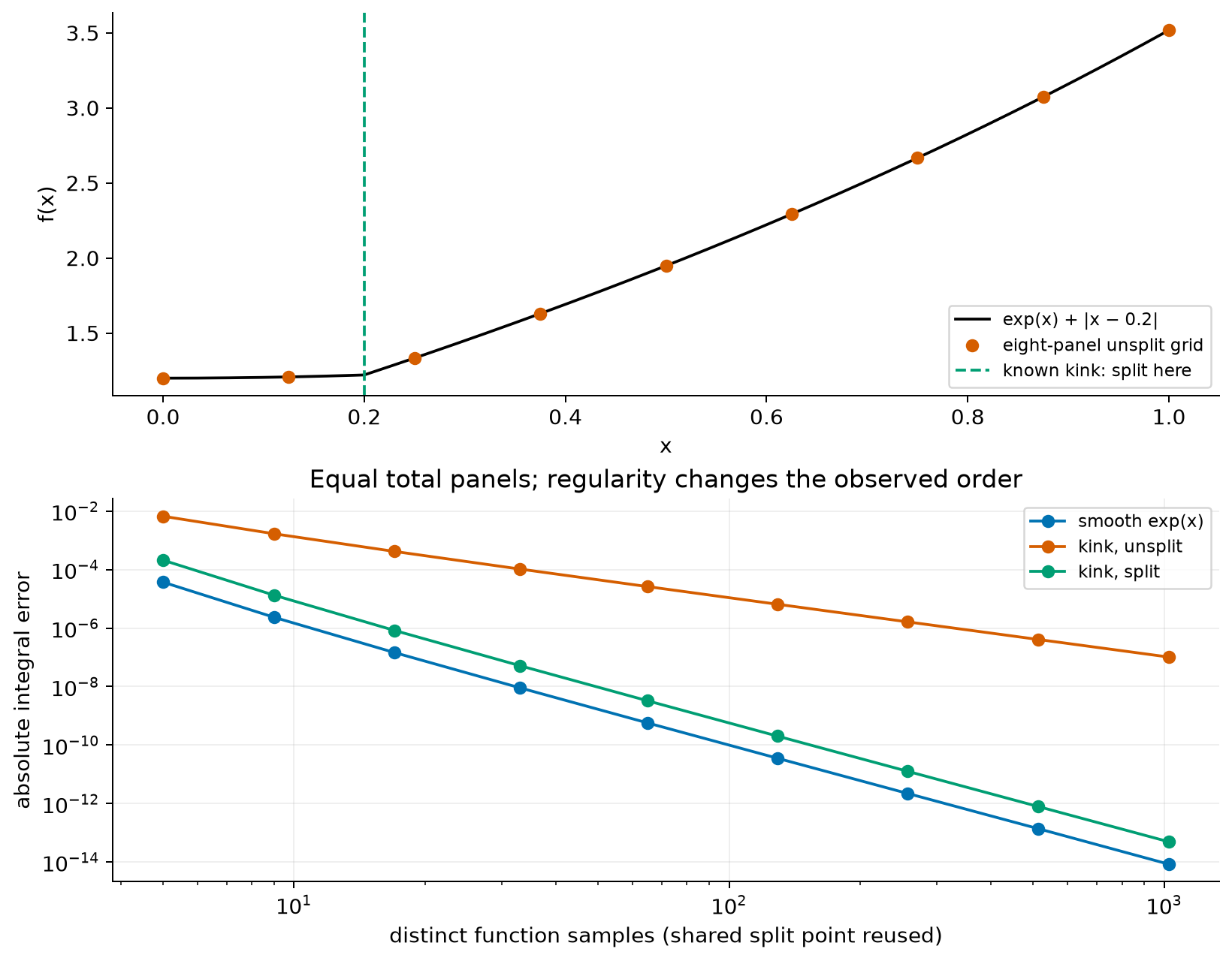
Figure 10:The unsplit calculation has a changing derivative inside one panel. Splitting puts that feature at the boundary of two smooth problems. The curves are measured against the stated analytic integrals. At the smallest errors, subtraction and summation round-off limit the interpretation of a fitted order.
The following are reference errors for from the plotted calculations. They are supplied data for interpreting convergence, not a Simpson implementation. The full comparison figure was generated separately.
# Reference errors; the comparison algorithms remain student implementation work.
panel_counts = np.array([16, 32, 64])
reference_errors = {
    "smooth": np.array([1.4559284666759709e-07, 9.102726128418226e-09, 5.689699822397642e-10]),
    "kink": np.array([0.0004165210738205083, 0.00010417576939314444, 2.6041097696882787e-05]),
    "split": np.array([8.310909613840067e-07, 5.198953223484182e-08, 3.250070435001362e-09]),
}

# Slices pair adjacent resolutions. log2(error ratio) measures the observed order.
for name, errors in reference_errors.items():
    orders = np.log2(errors[:-1] / errors[1:])
    print(f"{name:6s}: orders {orders[0]:.3f}, {orders[1]:.3f}")
smooth: orders 3.999, 4.000
kink : orders 1.999, 2.000
split : orders 3.999, 4.000
Do the observed orders identify the cause by themselves? State a comparison that would distinguish an incorrect weight pattern from insufficient regularity.
Answer: choose a test that separates the explanations
The smooth reference and polynomial-exactness checks test different properties of the implementation. Passing them, losing order only on the kinked function, and recovering the expected trend after splitting support the regularity explanation. A single failed convergence ratio does not establish a bug. Splitting is effective here because each piece is smooth. It is not a universal repair for an endpoint singularity or branch point. Recheck the assumptions and the observed regime after any transformation.
Answer: a correct order can have an unexpected cause
No. On these particular grids, Simpson integrates exactly in exact arithmetic, even though the kink lies between nodes. The remaining error comes from and has its fourth-order trend. Moving the kink to breaks that special cancellation. Smoothness is a sufficient condition for the quoted theorem, not a fact we can infer from one convergence plot. A change in grid alignment is a useful discriminating check.
Transfer: what if the samples are measurements?
A measured spectrum supplies values at fixed wavelengths. Interpolating those same values onto a denser grid does not add measurements. A quadrature result can converge for that interpolant while the inferred band flux remains limited by measurement uncertainty or unresolved lines.
For a fixed weighted sum , a covariance model for the measurements gives
For independent errors with known standard deviations , this reduces to . These are statistical uncertainties, not truncation-error bounds. Values interpolated from the same data are correlated; treating them as additional independent measurements would invent information. The formula also does not account for an unobserved feature between samples.
Which action addresses each limitation: refining quadrature, obtaining more spectral samples, improving measurement precision, or revising the interpolation model? Explain what evidence would make you choose it.
Answer: distinguish the computed curve from the observed source
Refinement reduces numerical integration error for a chosen curve. More observations can resolve a missed feature; more precise observations can reduce measurement uncertainty. Changing interpolation changes the model between the observations and requires justification. Agreement among dense-grid integrals of one interpolant establishes none of those improvements by itself.
Project 2 applications: endpoints and branch points
The formal order of a rule is conditional. The following applications make the conditions visible before you put the rules in a more complicated model.
A removable endpoint in the Planck integral
After the substitution , the Planck integral includes
Near , , so the integrand tends to and its limiting
value is 0. The mathematical integrand is finite at the endpoint, but the
literal floating-point expression at x == 0 is 0.0 / 0.0, which is nan.
np.expm1(x) evaluates accurately for small nonzero x; it does not
make division by zero at exactly x == 0 valid.
For a vectorized integrand, assign the analytic endpoint value explicitly or
construct a grid that excludes the endpoint and account for the omitted interval.
Do not accept a quiet nan, and do not call a small lower cutoff harmless
without bounding its contribution. The upper limit is also a numerical choice:
replace infinity with a finite , then show that increasing no longer
changes the answer at the precision you claim. The exact value is a
test target for this dimensionless stage before dimensional constants enter.
A radial transit integral and a regression limit
For the limb-darkened stellar disk, the radial integrand contains the factor
where is stellar radius in units of , is the projected
separation in the same units, and is the occulted fraction of an
annulus. The numerical rule should receive this integrand as a callable; it
does not need a special transit branch inside simpson.
The limit makes the intensity uniform. In that limit, the numerical limb-darkened calculation must reproduce the uniform-disk result from Project
This is a regression test: an earlier analytic model defines a known behaviour of the newer numerical model.
What a change of variables repairs
At the geometric contact radii , the occulted-annulus factor has a square-root branch point. A fixed Simpson grid can therefore lose fourth-order convergence even though it is correct on smooth functions. Splitting the domain at a known contact point isolates the feature but leaves it at a Simpson endpoint, so splitting alone need not restore the order.
If the relevant local behaviour is , set on that panel. Then
which is smooth at . The substitution changes both the variable and the Jacobian; omitting changes the integral. In Project 2, measure the order after the substitution rather than assuming that a mathematically plausible transformation restored it.
Real Application: Galaxy Luminosity from Spectrum
Astronomers measure galaxy spectra as discrete samples at wavelengths with fluxes . Under an isotropic nearby-source model, the luminosity in the measured wavelength band is:
Challenges
Irregular wavelength spacing from different instruments
Noise in flux measurements
Missing data from atmospheric absorption
Emission lines need high resolution
Solution Strategy
For irregular spacing, use trapezoidal rule with variable h:
def integrate_spectrum(wavelengths, fluxes):
    """Integrate spectrum with irregular spacing"""
    total = 0
    for i in range(len(wavelengths) - 1):
        dλ = wavelengths[i+1] - wavelengths[i]
        f_avg = (fluxes[i+1] + fluxes[i]) / 2
        total += dλ * f_avg
    return total
A gap bridged by this calculation assumes a straight-line interpolant across the missing interval. It does not establish the unobserved flux there. The finite-band result is not a bolometric luminosity without information about wavelengths outside the band.
For an emission line, choose the sampling density from the required integrated flux accuracy and the line shape; a fixed number of points per width is a starting diagnostic, not a guarantee.
Choosing the Right Integration Method
Method Comparison Summary
| Method | Order | Pros | Cons | Best For |
|---|---|---|---|---|
| Rectangle | on smooth functions | Simple; monotone left/right sums can bound an integral | More samples may be needed for a target | Baseline approximation, one-sided sampling, or monotonicity bounds |
| Trapezoid | on a smooth uniform grid | Directly applies to tabulated values | Lower order than Simpson for smooth callables | Sampled or irregularly spaced data |
| Simpson | for sufficient smoothness | Accurate per evaluation on smooth problems | Needs even n; loses order at non-smooth features | Smooth theoretical functions |
| Gaussian | Exact through polynomial degree | Efficient when nodes can be chosen | Special nodes and weights | Smooth callable, controlled sampling |
| Monte Carlo | RMS | Rate does not explicitly depend on dimension | Variance can make the constant large | Many integration variables or an effective variance-reduction strategy |
Practical Guidelines
State the data model: do you have a callable or already sampled values, and is the spacing uniform?
Check regularity: plot the integrand and locate discontinuities, sharp features, and endpoints before assigning an order.
Measure convergence: refine only in a range where the expected trend is visible, then identify the round-off floor.
Compare cost fairly: use function evaluations for deterministic rules and independent trials plus RMS error for Monte Carlo.
Use library routines deliberately: in production, read the library routine’s sampling, tolerance, and failure contracts rather than assuming it implements the classroom rule.
Debugging Integration
Common integration bugs and their diagnosis:
| Symptom | Likely Cause | Fix |
|---|---|---|
| Error does not decrease with n | Bug, unresolved structure, invalid error model, or rounding | First test polynomial exactness, then inspect sample locations and change the refinement range |
| Error plateaus near a floating-point floor | Round-off dominance | Stop claiming refinement will help; reassess scaling or precision if the target remains unmet |
| Oscillating convergence | Grid alignment or unresolved features | Shift diagnostic samples, locate known features, and compare split and unsplit refinement |
| Simpson gives weird results | Odd n | Ensure even intervals |
| Negative result for positive f | Reversed limits, incorrect weights, or inappropriate dtype | Check orientation, weights, and sampled values; overflow produces non-finite results and needs scaling or a different representation |
| Monte Carlo results fluctuate | Ordinary sampling variation, rare events, correlation, or invalid variance model | Compare independent repeats with a justified standard-error model before selecting a repair |
Bridge to the next block
Quadrature and root finding are distinct problems. They share useful habits: state the approximation, check preconditions, measure convergence in a valid regime, and report a failure rather than inventing a result.
This block ends with an integral estimate and an error claim. Block 3 begins a different contract: finding a value where , with bracketing, derivative, and initial-guess failure modes that quadrature does not have.
Later ODE methods reuse the local-to-global error distinction, but their step acceptance and stability requirements are separate again.
Next: Block 3 — Root Finding and Stellar Inference