Step acceptance, stopping, and accuracy
Keep these three decisions separate:
| Decision | Root finding | Quadrature |
|---|---|---|
| Accept a proposal | A line search tests decrease; a hybrid tests a bracket-preserving proposal. | An adaptive method compares local estimates before accepting a panel. |
| Stop the algorithm | Check the declared bracket, residual, or step criterion and iteration budget. | Check the allocated estimated-error budget and refinement limits. |
| Trust the answer | Check physical root selection, conditioning, and independent cases. | Check sampling adequacy, smoothness assumptions, cancellation, and independent cases. |
The backtracking example illustrates one accepted Newton step, not a complete solve. Line search does not preserve a bracket. Levenberg regularization changes the direction itself. These extensions are conceptual context; Project 3 still implements only its specified bisection, Newton, and secant methods.
For nested calculations, an outer root solver acts on the function supplied by an inner calculation. Neither accepted steps nor smaller outer tolerances can remove a fixed quadrature or trajectory error. The investigation below gives a concrete example of that limit.
Module Summary
The diagram separates two task families. They share the need for an explicit contract and convergence evidence; one is not the inverse of the other.
Part 1 introduces root-finding methods for Block 3:
Bisection halves a continuous sign-change bracket.
Newton can converge quadratically near a simple root when its local assumptions and starting point are suitable.
Secant avoids an analytic derivative and has superlinear local convergence under suitable assumptions.
Hybrid methods combine safeguards with faster local steps.
Part 2 supplies the Project 2 quadrature methods and a conceptual comparison:
Left rectangles make panel construction and first-order global error visible.
Trapezoid and Simpson have global orders 2 and 4 for sufficiently smooth functions.
Adaptive Simpson estimates a local error from one panel and two panels.
Monte Carlo, an optional extension, reports an estimator and sampling uncertainty, not a deterministic convergence guarantee.
Use the same review questions for either task: What is being approximated? What regularity or sampling assumption is required? What error is measured? Which test can show that the requested tolerance is met?
The implementation details and convergence laws remain specific to the task.
Key Takeaways
A continuous sign change is the precondition for bisection’s bracketed convergence guarantee.
Newton’s quadratic local convergence requires a simple root, a usable derivative, and an iterate already in the local convergence region.
A nominally higher-order quadrature rule is not guaranteed to retain that order at a discontinuity, kink, unresolved oscillation, or noisy-data fit.
With independent finite-variance samples, Monte Carlo RMS error scales as ; its practical cost also depends on variance and sampler quality.
A refinement study tests an observed error law. It does not prove that an asymptotic law applies at every resolution.
Richardson extrapolation requires a known leading error form and a regime in which that form is visible.
Investigation: an integral inside a root problem
Consider a dimensionless accumulated amount
We want the location where , so the root residual is . The integral measures an accumulated quantity; the root solver finds the position where that quantity reaches a target. These remain separate numerical tasks even when one calls the other.
An independent reference is available here: and . We use it to evaluate the evidence, not as an input to the numerical solvers.
Predict which tolerance matters
A reference calculation uses composite trapezoids for , then bisects its computed residual on . For each root tolerance it keeps the quadrature panel count fixed. Before looking at the results, predict:
Will a root half-width tolerance of 10-10 necessarily locate to 10-10?
What should happen when we keep that tolerance fixed but increase the number of quadrature panels?
Which information would let us bound the final position error?
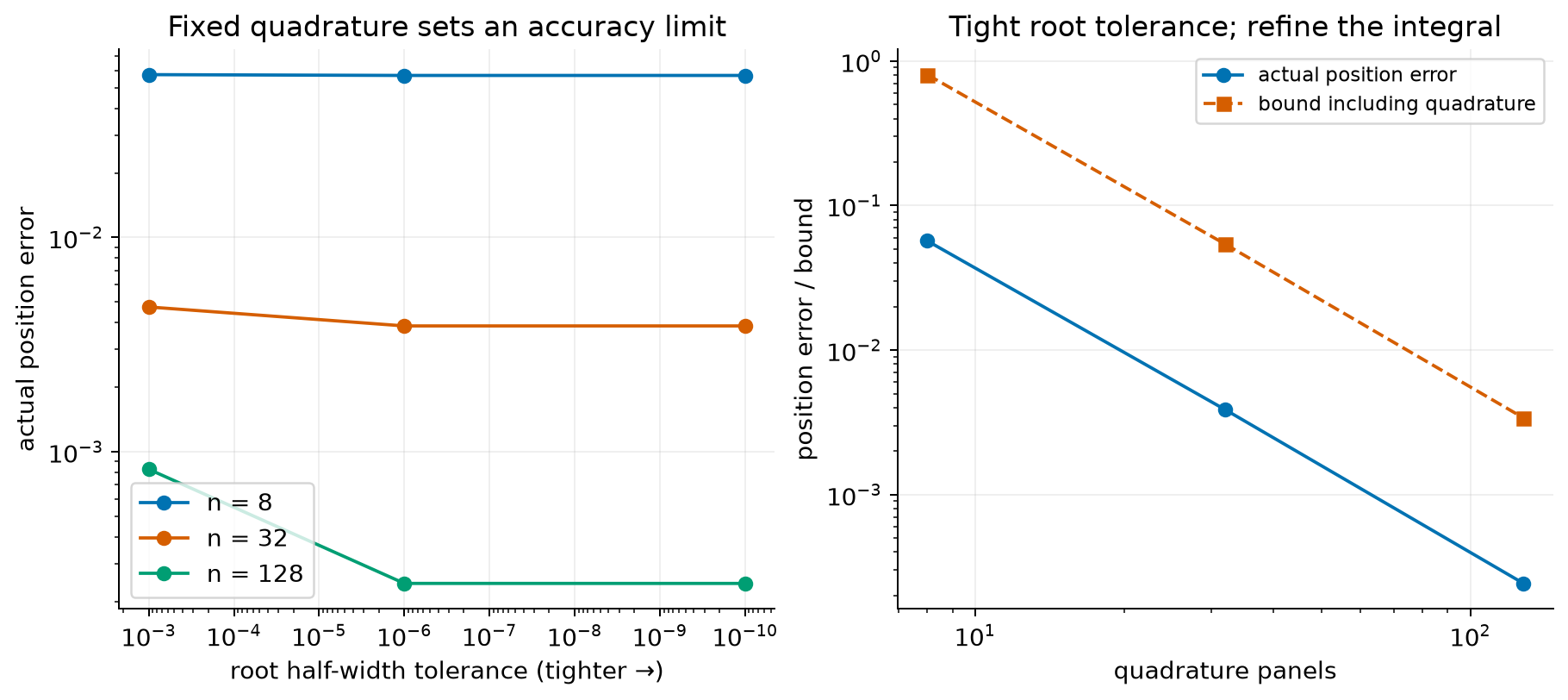
Figure 1:Each curve in the left panel solves a different fixed-resolution approximation to the integral. A narrow bracket for that approximate function is not a narrow bracket for the exact function. The right panel fixes the root tolerance and compares actual error with a conservative bound including quadrature error. All quantities are dimensionless.
Derive the shared error budget
Let be the computed residual and suppose a justified bound at the returned position satisfies
Assume the exact root and lie in an interval where is continuously differentiable and . The mean value theorem and triangle inequality give
and therefore
The two terms in the numerator have the residual’s units. Dividing by a slope converts them into position units. The first term describes how closely the computed equation was solved; the second describes how closely that equation approximates the intended one.
Here on , so we may use . For uniform trapezoid panels on , the integrand has , giving the exact-arithmetic bound
This bound is conservative; it uses the largest second derivative on every panel and the smallest residual slope on the full root-search interval. Floating-point evaluation and accumulation errors must also be included if they are material. In this example their scale is small relative to the displayed margins. If comes from an adaptive estimator instead of a proven bound, the final allowance is an estimate too.
import numpy as np

# Recorded reference results at root half-width tolerance 1e-10.
# Columns: quadrature panel count, returned position, computed residual magnitude.
reference_runs = np.array([[8, 2.2456068421597593, 9.704459458248493e-13], [32, 2.2987243363750167, 1.929789661403447e-12], [128, 2.302342479757499, 2.7243762801276716e-12]])
n_panels = reference_runs[:, 0].astype(int)
positions = reference_runs[:, 1]
computed_residuals = reference_runs[:, 2]
quadrature_bounds = positions**3 / (12*n_panels**2)
position_bounds = (computed_residuals + quadrature_bounds) / np.exp(-4)
actual_errors = np.abs(positions - np.log(10))

for n, residual, error, bound in zip(n_panels, computed_residuals, actual_errors, position_bounds):
    print(f"n={n:3d}: residual={residual:.2e}, position error={error:.2e}, bound={bound:.2e}")
n= 8: residual=9.70e-13, position error=5.70e-02, bound=8.05e-01
n= 32: residual=1.93e-12, position error=3.86e-03, bound=5.40e-02
n=128: residual=2.72e-12, position error=2.43e-04, bound=3.39e-03
The printed residual can be tiny while the position error is much larger. For a desired absolute position error , the bound suggests requiring . An equal split is one possible budget, not a universal optimum: the relative costs of reducing the two contributions determine a sensible allocation.
A subtle consequence: even the signs can be uncertain
If has absolute error bounded by , its sign is certified positive only when , and certified negative only when . Otherwise the allowed interval includes zero. A sign change in uncertain computed values alone cannot certify a bracket for . In the reference calculation, bisection narrows the approximate equation; the shared budget is the additional check against the exact equation.
Answer: which computation should receive more work?
A narrow bracket controls position for the function whose signs it reliably tracks. At fixed quadrature resolution, tightening that bracket eventually solves the approximate equation more precisely without improving the intended answer. If quadrature dominates the budget, refine the integral and check the change in the root. If the residual term dominates, refine the root solve. If function signs remain uncertain, improve their evaluation or retain that uncertainty; do not discard half an exact-function bracket using an uncertified sign. The analytic reference lets us test these claims in this example, but the argument identifies what information is needed when no reference is known.
Transfer: report only the claim your evidence supports
A collaborator reports: “The solver converged at tolerance 10-10.” Write a replacement explanation naming the target quantity, both approximation errors, the assumption converting residual to position, and one comparison that could falsify the claimed accuracy. If the target amount 0.9 also has a known absolute uncertainty, explain where that additional term belongs in the budget.
Reasoning to check against
The tolerance must name its quantity and units. A residual or approximate-bracket tolerance alone is insufficient. Bound or estimate the integral error, account for any uncertainty in the target amount, and divide their combined residual allowance by a valid slope lower bound. Compare roots from independently tighter quadrature while controlling root-solver error. Agreement is supporting evidence; it is not a replacement for the assumptions underlying a rigorous bound.
Looking Forward
For the current sequence:
Project 2: implement
rectangle,trapezoid, andsimpsonin a Python module; test their contracts and convergence; then add adaptive Simpson, and substitution. Monte Carlo has no assigned implementation, test, figure, or written response.Project 3: use root-finding methods and introduce the
Starclass.Later: distinguish quadrature from time-stepping methods for ODEs.
Before moving on, be able to name the quantity, state the rule’s preconditions, and show a test or convergence result for an implementation.
Quick Reference Tables
Root Finding Methods
| Method | Formula | Convergence | Iterations for ε | When to Use |
|---|---|---|---|---|
| Bisection | Interval width halves | for width | Continuous sign-change bracket | |
| Newton | Quadratic locally near a simple root | Problem-dependent | Derivative and suitable initial guess | |
| Secant | Superlinear locally | Problem-dependent | No analytic derivative; suitable starting pair |
Integration Methods
| Method | Local Error | Global Error | Function Evals | Best For |
|---|---|---|---|---|
| Left rectangle | Baseline rule; one-sided panels | |||
| Trapezoid | Smooth callable or tabulated data | |||
| Simpson | ; even | Smooth callable with even panel count | ||
| Gauss-Legendre | Exact through degree for nodes | Depends on the integrand and interval mapping | Smooth integrands; extension beyond Project 2 | |
| Monte Carlo | — | RMS with independent finite-variance samples | High-dimensional or irregular domains when sampling is practical |
Method Selection Guide
| If your problem has... | Use this method | Because... |
|---|---|---|
| Continuous sign-change bracket | Bisection | Preserves a bracket while reducing its width |
| Root with an expensive derivative | Secant or a safeguarded method | Avoids analytic derivative evaluation |
| Smooth one-dimensional integral | Simpson | Fourth-order global error after verifying the regime |
| Tabulated data | Trapezoid | Uses measured endpoint values without inventing a global interpolant |
| High-dimensional or irregular-domain integral | Monte Carlo candidate | Rate avoids tensor-grid scaling; compare variance and sampling cost |
| Several possible zeros | Use physical constraints, scan, and investigate candidates | A sign scan can miss tangencies or several crossings within a cell; one bracket need not isolate one root |
| Near machine precision | Reformulate and inspect error scale | More refinement may not improve a floating-point result |
Common Failure Modes and Fixes
| Problem | Symptom | Solution |
|---|---|---|
| Newton step is unstable or uninformative | Safeguard the step or use a bracketed method | |
| No sign change | Bisection cannot start | Scan the domain or use a method with different assumptions |
| Oscillatory integrand | Poor or misleading convergence | Resolve the shortest wavelength, split intervals, and verify refinement |
| High-dimensional integral | Tensor grid cost grows rapidly | Compare Monte Carlo, importance sampling, or problem-specific structure |
| Odd for Simpson | Project 2 contract is violated | Raise ValueError; do not silently alter the rule |
| Round-off dominance | Convergence plateau | Report the plateau and reconsider the scale or formulation |
Glossary
Adaptive quadrature: An integration method that estimates local error and subdivides intervals selectively. The estimate and stopping rule are part of the method contract.
Bisection method: A root-finding algorithm that repeatedly halves an interval containing a sign change. For a continuous function, the interval width is halved at every iteration.
Bracketing: Maintaining opposite endpoint signs on an interval. Continuity on that interval is required for the Intermediate Value Theorem to guarantee a root.
Catastrophic cancellation: Severe loss of significant digits when subtracting nearly equal floating-point numbers.
Condition number: A measure of how input perturbations affect an output. For a simple scalar root , describes the sensitivity of the root to an additive perturbation of the function value; its units depend on the problem’s variables.
Iteration order: A local relation between successive root errors. This differs from quadrature refinement order, , which compares different grid spacings at fixed integration limits. In both cases the stated regime and a nonzero leading term matter.
Curse of dimensionality: Rapid growth in the number of grid cells needed to resolve each additional dimension. The practical limit depends on resolution, structure, and computational budget; it is not a fixed dimension threshold.
Gaussian quadrature: A quadrature rule using nodes and weights chosen from an orthogonal-polynomial family. An -node Gauss-Legendre rule is exact for polynomials through degree on its reference interval.
Hybrid method: Algorithm combining multiple approaches, like Brent’s method mixing bisection’s reliability with interpolation’s speed for robust root finding.
Ill-conditioned: A problem in which small input perturbations can cause a large output change. Rapid oscillation creates a resolution problem; it is not by itself a condition-number statement.
Intermediate Value Theorem: If f is continuous on [a,b] and k is between f(a) and f(b), then there exists c [a,b] where f(c) = k; strictly intermediate values occur in (a,b).
Interpolation: Approximating a function between known points using simpler functions (lines for secant method, parabolas for Simpson’s rule).
Kepler’s equation: Transcendental equation E - e·sin(E) = M relating eccentric anomaly E to mean anomaly M for elliptical orbits. Classic root-finding application.
Lagrange points: Five equilibrium configurations of the circular restricted three-body problem. A spacecraft mission near one models an orbit in a rotating frame; the physical coordinate and stability conventions must be specified.
Linear convergence: Asymptotically the error decreases by a constant factor below one. Bisection halves a guaranteed interval-width bound; its actual midpoint error need not decrease by exactly one half.
Monte Carlo integration: A statistical estimator based on random samples. With independent finite-variance samples, its root-mean-square error scales as . Its suitability depends on variance, sampling method, dimensional structure, and cost.
Newton-Raphson method: A root-finding method using a tangent-line update. It has quadratic local convergence near a simple root under suitable smoothness and initialization assumptions.
Quadratic convergence: A local error law of the form . Newton’s method has this behavior near a simple root when its assumptions hold.
Quadrature: Numerical integration — approximating continuous integrals with discrete sums. From Latin “quadratura” meaning squaring, originally finding square with same area as curve.
Richardson extrapolation: Using results at different resolutions to cancel leading error terms, achieving higher accuracy from lower-order methods.
Root/Zero: A value for which . In physics, it can represent an equilibrium or an event location. An extremum is a root of a derivative only when that derivative exists and is the quantity being solved.
Secant method: Root-finding using line through two points instead of tangent. Achieves superlinear convergence (order 1.618, the golden ratio) without needing derivatives.
Simpson’s rule: Integration using parabolic interpolation through consecutive triplets of points. Achieves fourth-order accuracy despite using only quadratic polynomials.
Superlinear convergence: . Quadratic convergence belongs to this category; the secant method has the particular local order under its assumptions.
Transcendental equation: An equation involving functions such as sine, exponential, or logarithm. Many require numerical solution; special cases can have explicit answers.
Trapezoidal rule: Integration by connecting consecutive data points with straight lines. It is second-order accurate for a sufficiently smooth uniform grid; for measured data, it is a defined interpolation choice rather than a guarantee about an unknown underlying curve.
Well-conditioned: A problem whose output is relatively insensitive to the specified input perturbations and scaling. Algorithmic stability concerns how the numerical procedure propagates its own errors. A well-conditioned problem can still be evaluated by an unstable algorithm.
For Project 2, use the quadrature contract and its tests. Root-finding
implementations and the Star class enter in Project 3.