Learning objectives
By the end of this chapter, you will be able to:
1. Diagnose Python error messages by systematically analyzing tracebacks and exception types to identify bugs efficiently
2. Implement try/except blocks to gracefully handle expected failures in file I/O, network access, and data processing
3. Design input validation strategies using guard clauses, type checking, and domain constraints for scientific data
4. Apply assertions to document assumptions, verify mathematical properties, and catch numerical instabilities
5. Transform print-based debugging into structured logging with timestamps, severity levels, and persistent records
6. Create comprehensive test suites that verify known values, mathematical properties, edge cases, and regression scenarios
7. Debug code systematically using scientific method, diagnostic checkpoints, and hypothesis-testing approaches
8. Evaluate how errors propagate through scientific calculations and implement appropriate safeguards for numerical stability
Prerequisites
Before starting this chapter, verify you can:
Write and call functions with parameters (Chapter 5)
Work with NumPy arrays and array operations (Chapter 7)
Create plots with Matplotlib (Chapter 8)
Use if/else statements and loops (Chapter 3)
Work with lists and dictionaries (Chapter 4)
Read a traceback and identify the operation that raised an exception
Self-Assessment Diagnostic
Test your readiness by predicting what happens in each case:
# Question 1: What error will this produce?
data = [1, 2, 3]
print(data[3])

# Question 2: What result do you expect, and what does the computer store?
import numpy as np
values = np.array([1e16, 1.0, -1e16])
computed_sum = np.sum(values)

# Question 3: Will this file operation work?
with open('nonexistent.txt', 'r') as f:
    content = f.read()

# Question 4: What happens with this calculation?
def parsecs_to_lightyears(parsecs):
    return parsecs * 3.26156

distance = parsecs_to_lightyears("10")  # String instead of number
Self-Assessment Answers
IndexError: list index out of range (lists are 0-indexed, so valid indices are 0, 1, 2)
Loss of significance: Mathematically, the sum is 1.0. In ordinary float64 arithmetic the middle
1.0can be lost when it is added to1e16, so this ordering commonly produces 0.0. The result is finite, but it does not preserve the small contribution. This is a precision question, not evidence that every large-dynamic-range calculation is unstable.FileNotFoundError: The file doesn’t exist
TypeError: Can’t multiply string by float
If you struggled with these, review the prerequisite chapters first!
Why failures are evidence
Programs fail, and a useful failure exposes enough context to diagnose the problem. In scientific computing, validation and tests are ways to preserve a claim about behavior—not markers that someone has reached a more professional identity.
Think back to the simple functions we wrote in earlier chapters. In Chapter 5, we created calculate_mean(values) without checking if values was empty. In Chapter 7, we processed NumPy arrays without verifying they contained valid numbers. In Chapter 8, we plotted data assuming it was always plottable. Real scientific data breaks all these assumptions: sensors have failures producing NaN values, instruments have glitches creating outliers, and experiments can be interrupted leaving incomplete datasets.
Real failures make the stakes concrete, but they also resist single-cause morals. NASA’s Mars Climate Orbiter was lost after a failure to translate English and metric units; the Hubble mirror’s spherical aberration was traced to a lens-spacing error in a test device; and Ariane 501 failed shortly after launch and prompted an independent inquiry. Each case involved technical details, interfaces, review practices, and organizational decisions—not merely one missing if statement. This chapter gives you small, inspectable habits that contribute to those larger systems of evidence.
This chapter teaches you defensive programming—writing code that anticipates problems and handles them gracefully. You’ll learn to read error messages like a detective reading clues, understanding not just what went wrong but why and where. You’ll implement try/except blocks that catch expected errors like missing files or network timeouts without crashing your entire pipeline. You’ll validate inputs at function boundaries, checking that values are reasonable and arrays contain actual numbers. You’ll use assertions to verify internal invariants during development. When execution records and severity levels matter, you’ll use logging rather than scattered diagnostic prints. Finally, you’ll write tests that make stated behavior reproducible. A passing test demonstrates that stated behavior under stated conditions; it does not by itself establish physical adequacy, calibration, or scientific validity.
9.1 Understanding Error Messages
Error messages are Python’s way of communicating what went wrong during code execution. They’re structured reports that tell you the type of problem, where it occurred, and often hint at how to fix it. Learning to read them transforms debugging from frustrating guesswork into systematic detective work.
Your First Error Message
Let’s start with a simple temperature calculation that goes wrong:
# Temperature conversion
def kelvin_to_celsius(kelvin):
    """Convert temperature from Kelvin to Celsius."""
    return kevlin - 273.15  # Typo: 'kevlin' not 'kelvin'

# Try to use it
temp_k = 210  # Temperature in Kelvin
temp_c = kelvin_to_celsius(temp_k)
This produces a structured error message:
Traceback (most recent call last):
  File "temp.py", line 7, in <module>
    temp_c = kelvin_to_celsius(temp_k)
  File "temp.py", line 3, in kelvin_to_celsius
    return kevlin - 273.15
NameError: name 'kevlin' is not defined
Read error messages from bottom to top:
Error Type (bottom line):
NameErrortells you the category. A NameError means Python encountered a variable name it doesn’t recognize.Error Message: “name ‘kevlin’ is not defined” explains specifically what’s wrong—Python is looking for a variable called ‘kevlin’ but can’t find it in the current namespace.
Location (lines above): Shows exactly where the error occurred—file “temp.py”, line 3, inside function
kelvin_to_celsius.Call Stack (traceback): The traceback shows the sequence of function calls. Like following a trail, it shows that line 7 called the function, which failed at line 3.
Common Error Types in Scientific Computing
Let’s understand the exception types you’ll encounter most in scientific code:
# TypeError: Operating on wrong type
import numpy as np

# Common in data processing
def calculate_exposure_time(header):
    """Extract exposure time from header."""
    exptime = header['EXPTIME']  # Might be string "300.0" not float
    return exptime * 1.05  # TypeError if string!

# ValueError: Right type, wrong value
def calculate_magnitude(flux):
    """Convert flux to magnitude."""
    if flux <= 0:
        raise ValueError(f"Flux must be positive, got {flux}")
    return -2.5 * np.log10(flux)

# IndexError: Accessing beyond array bounds
def get_pixel_value(image, x, y):
    """Get pixel value."""
    return image[y, x]  # IndexError if x,y outside image!

# KeyError: Missing dictionary key
def process_observation(obs_dict):
    """Process observation metadata."""
    ra = obs_dict['RA']  # KeyError if 'RA' missing
    dec = obs_dict['DEC']
    return ra, dec
Understanding Error Propagation in Pipelines
In scientific data pipelines, one error can corrupt everything downstream:
def process_spectrum(wavelength, flux):
    """Complete spectroscopic reduction pipeline."""

    # Step 1: Calibration - a NaN wavelength propagates through the arithmetic.
    calibrated_wave = wavelength - 0.5  # Wavelength calibration offset

    # Step 2: Normalize - fails if flux has zeros or negative
    continuum = np.median(flux)
    if continuum <= 0:
        raise ValueError("Cannot normalize: continuum is non-positive")
    normalized_flux = flux / continuum

    # Step 3: Measure lines - fails if arrays mismatched
    if len(calibrated_wave) != len(normalized_flux):
        raise ValueError("Wavelength and flux arrays must match")

    # Step 4: Calculate equivalent width
    ew = np.trapz(1 - normalized_flux, calibrated_wave)

    return ew

# One bad value ruins everything
wave = np.array([6500, 6550, np.nan, 6650])  # NaN from bad pixel
flux = np.array([0.8, 0.6, 0.7, 0.9])
result = process_spectrum(wave, flux)  # Propagates NaN through everything!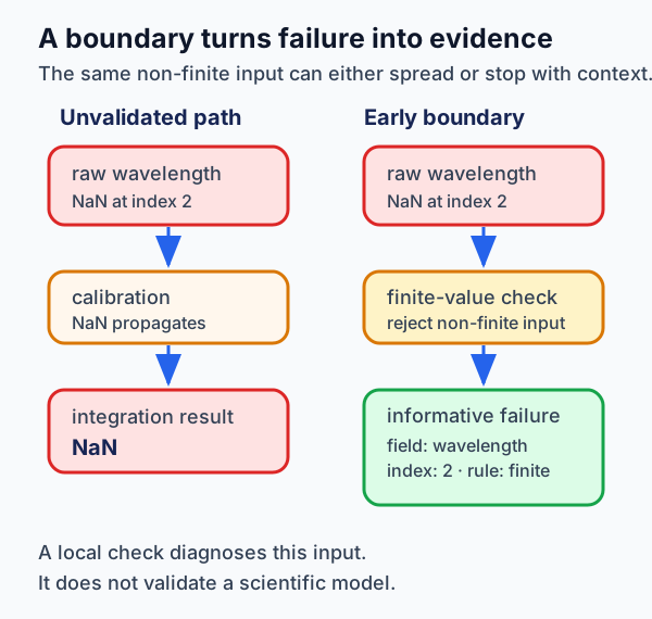
Figure 1:An early boundary turns a corrupting value into a local, reportable diagnostic.
What to notice: the check establishes a bounded software fact about this input. It does not establish calibration quality, physical validity, or adequacy of the scientific model.
9.2 Handling Errors with Try/Except
Sometimes errors are expected: files might be missing, network connections might timeout, or data might be corrupted. Try/except blocks let your program handle these situations gracefully instead of crashing during a critical operation.
Basic Try/Except Structure
import math

def read_magnitude(star_id, catalog):
    """Safely read stellar magnitude from catalog."""
    try:
        # Convert at the boundary instead of returning an unchecked string.
        magnitude = float(catalog[star_id]['mag'])
        if not math.isfinite(magnitude):
            raise ValueError("Magnitude must be finite")
        return magnitude
    except KeyError:
        # Star not in catalog
        print(f"Warning: Star {star_id} not in catalog")
        return None
    except (TypeError, ValueError):
        # Magnitude might be string 'variable' or 'saturated'
        print(f"Warning: Non-numeric magnitude for {star_id}")
        return None
Building Robust File Readers
Data files are fundamental in scientific computing. The following static example requires Astropy; it illustrates a boundary contract rather than a complete FITS quality-control pipeline.
from astropy.io import fits
import numpy as np

def read_fits_image(filename, extension=0):
    """
    Robust FITS file reader for astronomical images.

    Parameters
    ----------
    filename : str
        Path to FITS file
    extension : int
        HDU extension number (0 for primary)

    Returns
    -------
    data : ndarray or None
        Image data if successful
    header : dict or None
        FITS header if successful
    """
    try:
        # Open FITS file
        with fits.open(filename) as hdul:
            data = hdul[extension].data
            header = hdul[extension].header

            # Validate the boundary contract before numerical inspection.
            if data is None:
                raise ValueError("No data in FITS extension")
            data = np.asarray(data)
            if not np.issubdtype(data.dtype, np.number):
                raise ValueError(f"Expected numeric image data, got {data.dtype}")

            n_nonfinite = np.count_nonzero(~np.isfinite(data))
            if n_nonfinite > 0:
                print(f"Warning: {n_nonfinite} non-finite pixels found")

            # Check if image is saturated
            if 'SATURATE' in header:
                saturation = header['SATURATE']
                n_saturated = np.count_nonzero(data >= saturation)
                if n_saturated > 0:
                    print(f"Warning: {n_saturated} saturated pixels")

            return data, header

    except FileNotFoundError:
        print(f"Error: FITS file {filename} not found")
        return None, None

    except OSError as e:
        print(f"Error: Cannot read {filename} - may be corrupted")
        print(f"Details: {e}")
        return None, None

    except ValueError as e:
        print(f"Error: {filename} violates this reader's data contract: {e}")
        return None, None

    except (KeyError, IndexError) as e:
        print(f"Error: Extension {extension} not found in {filename}")
        return None, None
Handling Network Communication Errors
When downloading data or accessing remote resources, network issues are common:
import time

def download_data(data_id, max_retries=3, sleep=time.sleep):
    """
    Download data with automatic retry.

    Simulates downloading from remote archive.
    """
    for attempt in range(max_retries):
        try:
            # Simulate download attempt
            if attempt < 2:  # Simulate failures
                raise ConnectionError("Network timeout")

            # Successful download
            data = f"Data_{data_id}_content"
            return data

        except ConnectionError as e:
            wait_time = 2 ** attempt  # Exponential backoff
            print(f"Attempt {attempt + 1} failed: {e}")

            if attempt < max_retries - 1:
                print(f"Retrying in {wait_time} seconds...")
                sleep(wait_time)
            else:
                print(f"Failed after {max_retries} attempts")
                raise  # Re-raise the exception

    return None

# Test the retry mechanism
try:
    # Inject a no-op sleeper for this deterministic demonstration. A real caller
    # uses the default time.sleep or a project-specific retry policy.
    data = download_data("sample_001", sleep=lambda seconds: None)
    print(f"Successfully downloaded: {data}")
except ConnectionError:
print("Download failed - check network connection")When NOT to Use Try/Except
Not all errors should be caught. Programming mistakes should fail loudly:
# BAD: Hiding programming errors
def calculate_schwarzschild_radius(mass):
    try:
        # Typo: 'masse' instead of 'mass'
        return 2 * 6.67e-11 * masse / (3e8)**2
    except:  # Never use bare except!
        return 0  # Hides the typo!

# GOOD: Only catch expected errors
def calculate_schwarzschild_radius_correct(mass):
    """Calculate Schwarzschild radius with validation."""
    if mass <= 0:
        raise ValueError(f"Mass must be positive, got {mass}")

    G = 6.67430e-11  # m^3 kg^-1 s^-2
    c = 299792458    # m/s

    # Let typos crash loudly!
    r_s = 2 * G * mass / c**2

return r_s9.3 Validating Inputs
The best error is one that never happens. Input validation checks data at function boundaries, catching problems before they corrupt results. This is crucial in scientific computing where bad data can mean retracted papers.
Validating Scientific Measurements
def validate_magnitude(mag, band='V', object_type='star'):
    """
    Validate magnitude measurements.

    Parameters
    ----------
    mag : float
        Apparent magnitude
    band : str
        Photometric band (U, B, V, R, I, etc.)
    object_type : str
        Type of object (star, galaxy, quasar)
    """
    if not np.isscalar(mag):
        raise TypeError("Magnitude must be one scalar measurement")
    mag = float(mag)
    if not np.isfinite(mag):
        raise ValueError(f"Invalid magnitude: {mag}")

    # These are survey-screening limits for this classroom example, not
    # universal physical limits. A real pipeline reads them from its survey
    # configuration and preserves a flag rather than silently discarding data.
    screening_limits = {
        'star': {'V': (-2, 35)},
        'galaxy': {'V': (5, 35)},
        'quasar': {'V': (5, 35)},
    }

    if object_type in screening_limits and band in screening_limits[object_type]:
        min_mag, max_mag = screening_limits[object_type][band]
        if not min_mag <= mag <= max_mag:
            raise ValueError(
                f"{object_type} {band}={mag} outside configured screening range "
                f"[{min_mag}, {max_mag}]"
            )

    return True

def validate_coordinates(ra, dec, system='icrs'):
    """
    Validate celestial coordinates.

    Parameters
    ----------
    ra : float
        Right ascension in degrees
    dec : float
        Declination in degrees
    system : str
        Coordinate system (icrs, fk5, galactic)
    """
    if not (np.isscalar(ra) and np.isscalar(dec)):
        raise ValueError("Coordinates must be finite scalar values in degrees")
    try:
        ra = float(ra)
        dec = float(dec)
    except (TypeError, ValueError) as exc:
        raise ValueError("Coordinates must be finite scalar values in degrees") from exc
    if not (np.isfinite(ra) and np.isfinite(dec)):
        raise ValueError("Coordinates must be finite scalar values in degrees")
    if system in ['icrs', 'fk5']:
        if not 0 <= ra < 360:
            raise ValueError(f"RA={ra} outside range [0, 360)")
        if not -90 <= dec <= 90:
            raise ValueError(f"Dec={dec} outside range [-90, 90]")
    elif system == 'galactic':
        # Galactic longitude and latitude
        if not 0 <= ra < 360:  # l
            raise ValueError(f"Gal. longitude={ra} outside range")
        if not -90 <= dec <= 90:  # b
            raise ValueError(f"Gal. latitude={dec} outside range")
    else:
        raise ValueError(f"Unsupported coordinate system: {system}")

return TrueValidating Simulation Inputs
For computational physics, validate physical constraints:
def validate_nbody_initial_conditions(
    positions, velocities, masses, min_separation_m=1e-3,
    newtonian_speed_limit_fraction=0.01,
):
    """
    Validate N-body simulation initial conditions.

    Checks for physical consistency and numerical stability.
    """
    # Convert to arrays
    pos = np.asarray(positions)
    vel = np.asarray(velocities)
    m = np.asarray(masses)

    try:
        min_separation_m = float(min_separation_m)
        newtonian_speed_limit_fraction = float(newtonian_speed_limit_fraction)
    except (TypeError, ValueError) as exc:
        raise ValueError("Model thresholds must be finite scalar values") from exc
    if not (np.isfinite(min_separation_m) and min_separation_m > 0):
        raise ValueError("Collision threshold must be finite and positive")
    if not (np.isfinite(newtonian_speed_limit_fraction)
            and 0 < newtonian_speed_limit_fraction < 1):
        raise ValueError("Newtonian speed boundary must be between 0 and 1")

    # Check shapes and finite values.
    n_bodies = len(m)
    if n_bodies < 2:
        raise ValueError("At least two bodies are required")
    if pos.shape != (n_bodies, 3):
        raise ValueError(f"Position shape {pos.shape} != ({n_bodies}, 3)")
    if vel.shape != (n_bodies, 3):
        raise ValueError(f"Velocity shape {vel.shape} != ({n_bodies}, 3)")

    if not (np.all(np.isfinite(pos)) and np.all(np.isfinite(vel)) and np.all(np.isfinite(m))):
        raise ValueError("Positions, velocities, and masses must be finite")

    # Check masses are positive.
    if np.any(m <= 0):
        raise ValueError(f"Negative or zero masses found")

    # Check for coincident particles (numerical singularity)
    for i in range(n_bodies):
        for j in range(i+1, n_bodies):
            separation = np.linalg.norm(pos[i] - pos[j])
            if separation < min_separation_m:
                raise ValueError(
                    f"Particles {i} and {j} are coincident "
                    f"or closer than {min_separation_m} m (separation={separation} m)"
                )

    # This is a modeling boundary, not a numerical-stability threshold.
    speeds = np.linalg.norm(vel, axis=1)
    c = 299792458  # m/s
    if np.any(speeds > newtonian_speed_limit_fraction * c):
        fast_particles = np.where(speeds > newtonian_speed_limit_fraction * c)[0]
        raise ValueError(
            f"Particles {fast_particles} exceed this Newtonian model's "
            f"speed boundary ({newtonian_speed_limit_fraction} c)"
        )

return True9.4 Using Assertions
Assertions verify that your code’s internal logic is correct. Think of them as automated sanity checks that catch bugs during development.
Python can disable assertions with optimization flags, so use ValueError (or
another explicit exception) for inputs supplied by a caller. Reserve assert
for an internal invariant whose failure means the program itself is wrong.
Assertions vs Validation
There’s a critical distinction:
def calculate_orbital_period(semi_major_axis, total_mass):
    """
    Calculate orbital period using Kepler's third law.

    Shows difference between validation and assertions.
    """
    # VALIDATION: Check external inputs
    if semi_major_axis <= 0:
        raise ValueError(f"Semi-major axis must be positive: {semi_major_axis}")
    if total_mass <= 0:
        raise ValueError(f"Total mass must be positive: {total_mass}")

    # Calculate period (Kepler's third law)
    import math
    G = 6.67430e-11  # m^3 kg^-1 s^-2

    period_squared = (4 * math.pi**2 * semi_major_axis**3) / (G * total_mass)
    period = math.sqrt(period_squared)

    # ASSERTION: Verify our calculation is sensible
    assert period > 0, "Period calculation gave negative result!"
    assert np.isfinite(period), "Period calculation gave a non-finite result!"

    # For Earth-Sun system, should be ~365 days
    if abs(semi_major_axis - 1.496e11) < 1e10 and abs(total_mass - 1.989e30) < 1e29:
        assert abs(period - 365.25*24*3600) < 1e7, "Earth orbit calculation wrong!"

    return period
Numerical Stability Assertions
Assertions are crucial for catching numerical instabilities in scientific algorithms:
def integrate_relative_orbit_leapfrog(
    r0, v0, m1, m2, dt, n_steps, min_separation_m=1e3,
    max_relative_energy_error=1e-6,
):
    """
    Integrate relative two-body motion using leapfrog.

    `r0` and `v0` are relative separation and relative velocity in SI units.
    The energy tolerance is a diagnostic contract chosen from a timestep
    refinement study; it is not a universal accuracy threshold.
    """
    G = 6.67430e-11

    if m1 <= 0 or m2 <= 0 or dt <= 0 or n_steps < 1:
        raise ValueError("Masses, timestep, and number of steps must be positive")
    if min_separation_m <= 0 or max_relative_energy_error <= 0:
        raise ValueError("Separation and energy-error thresholds must be positive")

    # Initial conditions for the relative-coordinate problem.
    r = np.array(r0, dtype=np.float64)
    v = np.array(v0, dtype=np.float64)
    if r.shape != (3,) or v.shape != (3,):
        raise ValueError("r0 and v0 must each have three components")

    initial_separation = np.linalg.norm(r)
    if initial_separation <= min_separation_m:
        raise ValueError("Initial separation is below the collision boundary")

    # The kinetic term for relative motion uses the reduced mass.
    reduced_mass = m1 * m2 / (m1 + m2)
    kinetic_initial = 0.5 * reduced_mass * np.linalg.norm(v)**2
    potential_initial = -G * m1 * m2 / initial_separation
    energy_initial = kinetic_initial + potential_initial
    if energy_initial == 0:
        raise ValueError("Use an absolute energy diagnostic for a zero-energy orbit")

    positions = [r.copy()]

    for step in range(n_steps):
        # Leapfrog integration
        r_mag = np.linalg.norm(r)

        if r_mag <= min_separation_m:
            raise ValueError(f"Separation below {min_separation_m} m at step {step}")

        # Update velocity (half step)
        a = -G * (m1 + m2) * r / r_mag**3
        v += a * dt/2

        # Update position (full step)
        r += v * dt

        # Update velocity (half step)
        r_mag = np.linalg.norm(r)
        a = -G * (m1 + m2) * r / r_mag**3
        v += a * dt/2

        positions.append(r.copy())

        # Periodic invariant check. A non-finite energy is a programming or
        # numerical failure; the tolerance is supplied by the caller.
        if step % 100 == 0:
            kinetic = 0.5 * reduced_mass * np.linalg.norm(v)**2
            potential = -G * m1 * m2 / np.linalg.norm(r)
            energy = kinetic + potential

            energy_error = abs((energy - energy_initial) / energy_initial)
            assert np.isfinite(energy_error), "Energy diagnostic became non-finite"
            assert energy_error < max_relative_energy_error, (
                f"Energy diagnostic exceeds {max_relative_energy_error:.1e}: "
                f"{energy_error:.2e}"
            )

    return np.array(positions)
The More You Know: Remote Diagnosis on Voyager 2
In 2010, Voyager 2 began returning corrupted science data. NASA/JPL engineers
compared the changed data pattern with expected behavior, isolated one changed
bit in onboard memory, and reproduced the effect on an Earth-based computer.
The episode was not a classroom assert story: it was remote diagnosis using
telemetry, a testable hypothesis, and a controlled comparison before a fix.
The transferable lesson is modest but powerful. A useful diagnostic record lets you ask what changed, relative to which expectation, under which configuration? It does not eliminate uncertainty; it makes a failure investigable.
Debug This!
This function is numerically finite at high redshift. What scientific boundary does it cross instead?
def luminosity_distance_matter_lambda(z, H0=70, OmegaM=0.3, OmegaL=0.7):
    """
    Calculate luminosity distance for given redshift.

    Flat matter-plus-dark-energy classroom model; distances are in Mpc.
    """
    from scipy import integrate

    if z < 0 or H0 <= 0 or OmegaM < 0 or OmegaL < 0:
        raise ValueError("Require z >= 0, H0 > 0, and non-negative densities")
    if not np.isclose(OmegaM + OmegaL, 1.0):
        raise ValueError("This flat model requires OmegaM + OmegaL = 1")

    # Hubble distance
    c = 299792.458  # km/s
    DH = c / H0

    # Comoving distance integral
    def E(z_prime):
        return np.sqrt(OmegaM * (1 + z_prime)**3 + OmegaL)

    # This integral is well behaved at z=1100 in float64.
    DC, error = integrate.quad(lambda zp: 1/E(zp), 0, z)
    DC *= DH

    # Luminosity distance
    DL = (1 + z) * DC

    assert DL > 0, f"Luminosity distance {DL} is negative!"
    assert np.isfinite(DL), f"Luminosity distance {DL} is non-finite!"

    return DL

# This produces a finite number at z=1100, but that does not make the model
# adequate for the CMB epoch.
# result = luminosity_distance_matter_lambda(1100)
Bug Explanation
There is no float64 overflow at : is only about 109. The boundary is physical. Radiation contributes materially near recombination, so a matter-plus-dark-energy model is not an adequate CMB-era distance model. The finite result only shows that this implementation evaluated its stated toy equation.
9.5 Logging as Diagnosis
Use logging when an execution record, severity level, or machine-readable
diagnostic matters. print() remains useful for a short interactive
exploration; logging is the better tool for a pipeline, service, or
long-running simulation whose history someone must inspect later.
From Local Messages to a Diagnostic Record
Configure handlers at an application entry point, not inside an importable library function. This static example uses a named logger and a deterministic synthetic image so its diagnostics can be reproduced:
import logging
import numpy as np

# Configure logging once at an application entry point.
logging.basicConfig(
    level=logging.INFO,
    format='%(asctime)s - %(name)s - %(levelname)s - %(message)s',
    handlers=[
        logging.FileHandler('data_pipeline.log'),
        logging.StreamHandler()  # Also print to console
    ]
)

logger = logging.getLogger('DataPipeline')

def process_image(image, dark_frame, flat_frame):
    """
    Process image with proper logging.

    Demonstrates logging at different severity levels.
    """
    image = np.asarray(image, dtype=float)
    dark_frame = np.asarray(dark_frame, dtype=float)
    flat_frame = np.asarray(flat_frame, dtype=float)
    if not (image.shape == dark_frame.shape == flat_frame.shape):
        logger.error("Image, dark frame, and flat frame must have the same shape")
        return None
    if not (np.all(np.isfinite(image)) and np.all(np.isfinite(dark_frame))):
        logger.error("Image and dark frame must contain only finite values")
        return None
    if not (np.all(np.isfinite(flat_frame)) and np.all(flat_frame > 0)):
        logger.error("Flat frame must be finite and strictly positive")
        return None

    logger.info(f"Starting image reduction: shape {image.shape}")

    # Saturation belongs to the detector's raw-count space, before calibration.
    saturation_level = 65535  # 16-bit detector counts
    n_raw_saturated = np.sum(image >= saturation_level)
    if n_raw_saturated > 0:
        logger.warning(f"{n_raw_saturated} saturated raw pixels detected")

    # Dark subtraction
    logger.debug(f"Dark frame statistics: mean={np.mean(dark_frame):.2f}")
    dark_subtracted = image - dark_frame

    # Negative values after dark subtraction can be ordinary measurement noise.
    # Preserve them; log the fact rather than silently changing the data.
    n_negative = np.sum(dark_subtracted < 0)
    if n_negative > 0:
        logger.info(f"Found {n_negative} negative pixels after dark subtraction")

    # Flat fielding
    flat_corrected = dark_subtracted / flat_frame

    # Outlier detection (simplified)
    median = np.median(flat_corrected)
    std = np.std(flat_corrected)
    n_outliers = np.sum(flat_corrected > median + 10*std)
    if n_outliers > 0:
        logger.info(f"Detected {n_outliers} potential outliers")

    logger.info("Image reduction complete")
    return flat_corrected

# Example usage with deterministic simulated data.
rng = np.random.default_rng(20260821)
image = rng.poisson(1000, (128, 128)).astype(float)
dark = rng.poisson(100, (128, 128)).astype(float)
flat = np.ones((128, 128)) + rng.normal(0, 0.1, (128, 128))

result = process_image(image, dark, flat)
Logging Long-Running Simulations
For simulations that run for days, logging provides crucial diagnostics. The following is pseudocode: it requires a simulation-specific timestep, energy diagnostic, and checkpoint writer. It deliberately does not invent a random “energy” to make a log look realistic.
import time
import math

def run_simulation(n_particles, n_steps, evolve_one_timestep, total_energy, save_checkpoint):
    """
    Run N-body simulation with progress logging.
    """
    sim_logger = logging.getLogger('Simulation')

    # Log simulation parameters
    sim_logger.info(f"Starting simulation: {n_particles} particles, {n_steps} steps")
    sim_logger.info(f"Memory estimate: {n_particles * 6 * 8 / 1e9:.2f} GB")

    # Simulation loop
    if n_steps < 1:
        raise ValueError("n_steps must be positive")
    checkpoint_interval = max(1, n_steps // 10)
    energy_initial = float(total_energy())
    if not math.isfinite(energy_initial) or energy_initial == 0:
        raise ValueError(
            "Relative energy drift requires a finite, non-zero initial energy; "
            "use an absolute diagnostic otherwise"
        )

    for step in range(n_steps):
        # Evolve system
        evolve_one_timestep()

        # Periodic logging
        if step % checkpoint_interval == 0:
            progress = 100 * step / n_steps
            energy_current = float(total_energy())
            if not math.isfinite(energy_current):
                raise ValueError("Energy diagnostic became non-finite")
            energy_drift = abs((energy_current - energy_initial) / energy_initial)

            sim_logger.info(
                f"Step {step}/{n_steps} ({progress:.1f}%): "
                f"Energy drift = {energy_drift:.2e}"
            )

            # Alert if energy conservation violated
            if energy_drift > 1e-4:
                sim_logger.warning(f"Large energy drift detected: {energy_drift:.2e}")

            # Save checkpoint
            if step % (checkpoint_interval * 5) == 0:
                save_checkpoint(f"checkpoint_{step:06d}.hdf5")
                sim_logger.info(f"Checkpoint saved at step {step}")

sim_logger.info("Simulation complete")9.6 Writing Simple Tests
Testing isn’t about proving perfection—it’s about checking a stated
behavior before it quietly becomes an assumption in later work. Put test files
named test_*.py beside your code and run them with python -m pytest.
pytest discovers functions named test_*; each test should arrange a known
state, act once, and assert the observable contract.
Testing Scientific Calculations
import numpy as np
import pytest

def magnitude_to_relative_flux(magnitude, zero_point=0):
    """Return flux relative to the supplied zero point, not physical flux units."""
    return 10**(-0.4 * (magnitude - zero_point))

def relative_flux_to_magnitude(relative_flux, zero_point=0):
    """Invert the relative-flux convention used above."""
    if relative_flux <= 0:
        raise ValueError(f"Relative flux must be positive, got {relative_flux}")
    return -2.5 * np.log10(relative_flux) + zero_point

def test_magnitude_conversions():
    """Test magnitude-flux conversions."""

    # Arrange / act / assert: zero magnitude maps to unit relative flux.
    assert magnitude_to_relative_flux(0) == pytest.approx(1.0)

    # 5 magnitudes = factor of 100 in flux
    assert magnitude_to_relative_flux(5) == pytest.approx(0.01)

    # Test 2: Round trip
    original_mag = 15.5
    relative_flux = magnitude_to_relative_flux(original_mag)
    recovered_mag = relative_flux_to_magnitude(relative_flux)
    assert recovered_mag == pytest.approx(original_mag)

    # Test 3: Mathematical properties
    mag1, mag2 = 10, 12
    flux1 = magnitude_to_relative_flux(mag1)
    flux2 = magnitude_to_relative_flux(mag2)
    flux_ratio = flux1 / flux2
    expected_ratio = 10**(0.4 * (mag2 - mag1))
    assert flux_ratio == pytest.approx(expected_ratio)

    # Test 4: Edge cases
    with pytest.raises(ValueError, match="positive"):
        relative_flux_to_magnitude(-1)
Testing Coordinate Transformations
import numpy as np

def test_coordinate_transformations():
    """Test coordinate transformations."""

    # Test RA/Dec to Cartesian
    def radec_to_cartesian(ra, dec):
        """Convert RA/Dec (degrees) to unit vector."""
        ra_rad = np.radians(ra)
        dec_rad = np.radians(dec)

        x = np.cos(dec_rad) * np.cos(ra_rad)
        y = np.cos(dec_rad) * np.sin(ra_rad)
        z = np.sin(dec_rad)

        return np.array([x, y, z])

    # Test 1: Cardinal directions
    # RA=0, Dec=0 should point to x-axis
    vec = radec_to_cartesian(0, 0)
    assert np.allclose(vec, [1, 0, 0]), "Vernal equinox wrong"

    # RA=90, Dec=0 should point to y-axis
    vec = radec_to_cartesian(90, 0)
    assert np.allclose(vec, [0, 1, 0]), "RA=90 wrong"

    # North celestial pole
    vec = radec_to_cartesian(0, 90)
    assert np.allclose(vec, [0, 0, 1]), "North pole wrong"

    # Test 2: Unit vector property
    for ra in [0, 45, 180, 270]:
        for dec in [-90, -45, 0, 45, 90]:
            vec = radec_to_cartesian(ra, dec)
            norm = np.linalg.norm(vec)
            assert abs(norm - 1.0) < 1e-10, f"Not unit vector: {norm}"

    print("✓ Coordinate transformation tests passed!")

test_coordinate_transformations()
Parameterized Boundaries, Determinism, and Convergence
Use parametrization when the same contract must hold at several boundaries. Use a local random generator when a test needs randomness, so a failure can be reproduced exactly. A convergence check supplies stronger numerical evidence than a single plausible-looking value.
import numpy as np
import pytest

@pytest.mark.parametrize("ra, dec", [(0, 0), (359.999, 90), (180, -90)])
def test_coordinate_bounds(ra, dec):
    assert 0 <= ra < 360
    assert -90 <= dec <= 90

def test_seeded_noise_is_reproducible():
    first = np.random.default_rng(20260821).normal(size=4)
    second = np.random.default_rng(20260821).normal(size=4)
    assert np.array_equal(first, second)

def euler_exponential(dt, final_time=1.0):
    """Solve y' = y, y(0) = 1 with a timestep that reaches final_time."""
    try:
        dt = float(dt)
        final_time = float(final_time)
    except (TypeError, ValueError) as exc:
        raise ValueError("dt and final_time must be finite and positive") from exc
    if not (np.isfinite(dt) and np.isfinite(final_time) and dt > 0 and final_time > 0):
        raise ValueError("dt and final_time must be finite and positive")
    n_steps = round(final_time / dt)
    if not np.isclose(n_steps * dt, final_time):
        raise ValueError("dt must divide final_time for this classroom example")
    y = 1.0
    for _ in range(n_steps):
        y += dt * y
    return y

def test_euler_refinement_reduces_error():
    exact = np.exp(1.0)
    coarse_error = abs(euler_exponential(0.1) - exact)
    fine_error = abs(euler_exponential(0.05) - exact)
    assert fine_error < coarse_error
Testing Edge Cases in Physics Calculations
import math
import pytest

def doppler_redshift_to_velocity(z, relativistic=True):
    """Convert a special-relativistic Doppler redshift to velocity in km/s."""
    try:
        z = float(z)
    except (TypeError, ValueError) as exc:
        raise ValueError("Doppler redshift must be a finite scalar") from exc
    if not math.isfinite(z) or z <= -1:
        raise ValueError("Doppler redshift must be finite and greater than -1")
    if relativistic:
        # Special relativistic formula
        c = 299792.458  # km/s
        return c * ((1 + z)**2 - 1) / ((1 + z)**2 + 1)
    else:
        # Non-relativistic approximation
        c = 299792.458
        return c * z

def test_redshift_velocity():
    """Test redshift-velocity conversions with edge cases."""

    c = 299792.458  # km/s

    # Test 1: Zero redshift = zero velocity.
    assert doppler_redshift_to_velocity(0) == pytest.approx(0)

    # Test 2: Small redshift - relativistic and non-relativistic agree
    z_small = 0.001
    v_rel = doppler_redshift_to_velocity(z_small, relativistic=True)
    v_nonrel = doppler_redshift_to_velocity(z_small, relativistic=False)
    assert v_rel == pytest.approx(v_nonrel, rel=1e-3)

    # Test 3: Speed of light limit
    z_large = 1000  # Very high redshift
    v = doppler_redshift_to_velocity(z_large)
    assert v < c, f"Velocity {v} exceeds speed of light!"

    # Test 4: Known values
    # z=1 should give v = 3c/5
    v_z1 = doppler_redshift_to_velocity(1)
    expected = 3 * c / 5
    assert v_z1 == pytest.approx(expected)

    # Test 5: Negative redshift (blueshift)
    z_blue = -0.001  # Small blueshift (like Andromeda)
    v_blue = doppler_redshift_to_velocity(z_blue)
    assert v_blue < 0, "Blueshift should give negative velocity"

    print("✓ Redshift velocity tests passed!")

test_redshift_velocity()
This is a Doppler-equivalent velocity convention. Do not use it as a general conversion from cosmological redshift to a unique recession velocity; that interpretation depends on the cosmological model and coordinates.
9.7 Debugging Strategies
Debugging is detective work. Instead of randomly changing code hoping it works, follow a systematic approach that mirrors the scientific method.
The Scientific Method of Debugging
import numpy as np
import pytest

def demonstrate_debugging_process():
    """Show systematic debugging of a cosmological calculation."""

    # THE PROBLEM: Hubble parameter calculation gives wrong result
    def buggy_hubble_parameter(z, H0=70, OmegaM=0.3, OmegaL=0.7):
        """Calculate H(z) - has a bug."""
        # E(z) = sqrt(OmegaM*(1+z)^3 + OmegaL)
        E_z = np.sqrt(OmegaM * (1+z)**3 + OmegaL * (1+z)**2)  # Bug here!
        return H0 * E_z

    # STEP 1: OBSERVE - use a nonzero case that distinguishes the models.
    z_test = 1
    result = buggy_hubble_parameter(z_test)
    expected = H0_expected = 70 * np.sqrt(0.3 * (1 + z_test)**3 + 0.7)
    print(f"Expected H({z_test}) = {expected:.2f}, got {result:.2f}")

    # STEP 2: HYPOTHESIZE - Form theories
    print("\nHypotheses:")
    print("1. H0 scaling wrong?")
    print("2. OmegaM term wrong?")
    print("3. OmegaL term wrong?")

    # STEP 3: EXPERIMENT - Test each component
    print(f"\nTesting components at z={z_test}:")

    z = z_test
    OmegaM, OmegaL = 0.3, 0.7

    # Test each term separately
    matter_term = OmegaM * (1+z)**3
    print(f"Matter term: {matter_term:.2f}")

    dark_energy_term = OmegaL * (1+z)**2  # Bug found!
    print(f"Dark-energy term: {dark_energy_term:.2f} (should be {OmegaL:.2f})")
    print(f"ERROR: Dark energy shouldn't have (1+z) dependence!")

    # STEP 4: FIX - Correct the bug
    def hubble_parameter_fixed(z, H0=70, OmegaM=0.3, OmegaL=0.7):
        """Fixed version."""
        E_z = np.sqrt(OmegaM * (1+z)**3 + OmegaL)  # Fixed!
        return H0 * E_z

    # Verify fix
    result_fixed = hubble_parameter_fixed(z_test)
    assert result_fixed == pytest.approx(H0_expected)
    print(f"\nFixed: H({z_test}) = {result_fixed:.2f} ✓")

demonstrate_debugging_process()
Diagnostic Checkpoints for Complex Pipelines
When debugging a long processing pipeline, record a small number of diagnostic checkpoints at meaningful boundaries. This is not literal binary search: it preserves evidence at each stage so a failing contract can be located and then investigated.
def debug_spectroscopy_pipeline(spectrum_file):
    """
    Debug a complex spectroscopy pipeline with diagnostic checkpoints.
    """

    # Add checkpoints at meaningful scientific boundaries.
    checkpoints = []

    # === FIRST HALF ===
    # Step 1: Read raw spectrum
    raw_spectrum = read_raw_spectrum(spectrum_file)
    checkpoints.append(("Raw read", validate_spectrum(raw_spectrum)))

    # Step 2: Wavelength calibration
    calibrated = wavelength_calibrate(raw_spectrum)
    checkpoints.append(("Wavelength cal", validate_spectrum(calibrated)))

    # Step 3: Flux calibration
    flux_cal = flux_calibrate(calibrated)
    checkpoints.append(("Flux cal", validate_spectrum(flux_cal)))

    # === MIDPOINT CHECKPOINT ===
    print("=== MIDPOINT CHECK ===")
    for name, valid in checkpoints:
        print(f"{name}: {'✓' if valid else '✗'}")

    # === SECOND HALF ===
    # Step 4: Continuum normalization
    normalized = normalize_continuum(flux_cal)
    checkpoints.append(("Continuum", validate_spectrum(normalized)))

    # Step 5: Redshift correction
    deredshifted = correct_redshift(normalized)
    checkpoints.append(("Redshift", validate_spectrum(deredshifted)))

    # Step 6: Line measurement
    lines = measure_lines(deredshifted)
    checkpoints.append(("Lines", lines is not None))

    # Final diagnostic
    print("\n=== FULL PIPELINE DIAGNOSTIC ===")
    for i, (name, valid) in enumerate(checkpoints):
        status = '✓' if valid else '✗ FAILURE HERE'
        print(f"Step {i+1}: {name:15} {status}")
        if not valid:
            print(f"  -> Problem isolated to step {i+1}: {name}")
            break

    return checkpoints

def validate_spectrum(spectrum):
    """Check if spectrum is valid."""
    if spectrum is None:
        return False
    if hasattr(spectrum, 'flux'):
        return np.all(np.isfinite(spectrum.flux))
    return True

# Placeholder functions
def read_raw_spectrum(f): return type('Spectrum', (), {'flux': np.ones(100)})()
def wavelength_calibrate(s): return s
def flux_calibrate(s): return s
def normalize_continuum(s): return s
def correct_redshift(s): return s
def measure_lines(s): return {'Ha': 6563}

# Test the debugging
result = debug_spectroscopy_pipeline("test_spectrum.fits")
Common Debugging Patterns in Scientific Computing
Recognize these common bugs in scientific code:
# Pattern 1: Unit Confusion
def buggy_schwarzschild_radius(mass_solar):
    """Bug: Mixing unit systems."""
    G = 6.67e-11  # SI units (m^3 kg^-1 s^-2)
    c = 3e8       # SI units (m/s)
    M = mass_solar  # BUT THIS IS IN SOLAR MASSES!
    return 2 * G * M / c**2  # Wrong units!

def fixed_schwarzschild_radius(mass_solar):
    """Fixed: Consistent units."""
    G = 6.67e-11  # SI
    c = 3e8       # SI
    M_sun = 1.989e30  # kg
    M = mass_solar * M_sun  # Convert to SI
    r_s = 2 * G * M / c**2  # meters
    return r_s / 1000  # Return in km for convenience

# Pattern 2: Array Index vs Physical Coordinate
def buggy_find_peak(image):
    """Bug: Confusing pixel index with position."""
    peak_idx = np.unravel_index(np.argmax(image), image.shape)
    # Returns (y_index, x_index) not (x_coord, y_coord)!
    return peak_idx  # Wrong order for most uses

def fixed_find_peak(image, pixel_scale=1.0):
    """Fixed: Clear about indices vs coordinates."""
    y_idx, x_idx = np.unravel_index(np.argmax(image), image.shape)
    # Convert to standard (x, y) coordinates; document pixel_scale units.
    x_coord = x_idx * pixel_scale
    y_coord = y_idx * pixel_scale
    return {'indices': (y_idx, x_idx),
            'coordinates': (x_coord, y_coord),
            'value': image[y_idx, x_idx]}

# Pattern 3: Cosmological Convention Confusion
def buggy_comoving_distance(z, H0=70):
    """Bug: Wrong convention for H0."""
    # Is H0 in km/s/Mpc or s^-1?
    c = 3e8  # m/s - WRONG for H0 in km/s/Mpc!
    return c * z / H0

def fixed_comoving_distance(z, H0=70):
    """Fixed: Clear about units."""
    c_km_s = 299792.458  # km/s to match H0 units
    # H0 in km/s/Mpc, returns distance in Mpc
return c_km_s * z / H0 # Simple approximation for small zPractice Exercises
Exercise 1: Robust Data Pipeline
Create a robust pipeline for processing data files:
Part A: Basic file handling (5 minutes)
def read_data_basic(filename):
    """
    Step 1: Handle missing or corrupted files.

    Should:
    - Return None, None if file doesn't exist
    - Return None, None if file is corrupted
    - Return data, header if successful
    """
    # Your code here
    pass
Part B: Add validation (10 minutes)
def read_data_validated(filename):
    """
    Step 2: Add data validation.

    Should additionally:
    - Check for NaN/Inf values
    - Verify required header keywords
    - Check if values are in expected range
    """
    # Build on Part A
    pass
Part C: Complete pipeline with logging (10 minutes)
def process_data_robust(filename, calibration=None):
    """
    Step 3: Complete processing pipeline.

    Should:
    - Read data with all validation
    - Apply calibration if provided
    - Log all operations and warnings
    - Return processed data or None if failed
    """
    # Complete implementation
    pass
Exercise 2: Physics Calculator with Full Validation
Build a robust physics calculator:
def calculate_distances(z, H0=70, OmegaM=0.3, OmegaL=0.7):
    """
    Calculate cosmological distances with full validation.

    Should:
    - Validate all inputs are in valid ranges
    - State that this classroom model is spatially flat and check
      `OmegaM + OmegaL` accordingly
    - Handle both scalar and array inputs for z
    - Use explicit validation for caller inputs and assertions only for an
      internal invariant
    - Return dict with luminosity_distance, angular_diameter_distance
    - Flag that a matter-plus-dark-energy model is not adequate for CMB-era
      redshift without radiation
    """
    # Your implementation here
    pass

# Test cases:
test_cases = [
    {'z': 0.1},                    # Nearby
    {'z': 1.0},                    # Typical
    {'z': 1100},                   # Require a model-boundary response
    {'z': -0.001},                 # Invalid (should raise error)
    {'z': [0.1, 0.5, 1.0]},       # Array input
]
Exercise 3: N-body Integrator Test Suite
Write comprehensive tests for this gravitational N-body integrator:
import numpy as np

def nbody_step(positions, velocities, masses, dt, G=6.67e-11):
    """
    Single step of N-body integration using leapfrog.

    Parameters
    ----------
    positions : array, shape (N, 3)
    velocities : array, shape (N, 3)
    masses : array, shape (N,)
    dt : float
        Timestep
    """
    positions = np.asarray(positions, dtype=float).copy()
    velocities = np.asarray(velocities, dtype=float).copy()
    masses = np.asarray(masses, dtype=float)
    n = len(masses)
    accelerations = np.zeros_like(positions, dtype=float)

    # Calculate accelerations
    for i in range(n):
        for j in range(n):
            if i != j:
                r = positions[j] - positions[i]
                r_mag = np.linalg.norm(r)
                if r_mag == 0:
                    raise ValueError("Collision: pairwise force is singular")
                accelerations[i] += G * masses[j] * r / r_mag**3

    # Leapfrog integration
    velocities += accelerations * dt/2
    positions += velocities * dt

    # Recalculate accelerations at new positions
    accelerations = np.zeros_like(positions, dtype=float)
    for i in range(n):
        for j in range(n):
            if i != j:
                r = positions[j] - positions[i]
                r_mag = np.linalg.norm(r)
                if r_mag == 0:
                    raise ValueError("Collision: pairwise force is singular")
                accelerations[i] += G * masses[j] * r / r_mag**3

    velocities += accelerations * dt/2

    return positions, velocities

def test_nbody_integrator():
    """
    Write comprehensive tests.

    Should test:
    - Two-body circular orbit (analytical solution exists)
    - Energy conservation over many steps
    - Momentum conservation
    - Handle collision (r -> 0)
    - Input arrays are not unexpectedly mutated
    - Benchmark separately on a declared workload; do not make runtime a
      machine-dependent unit-test assertion
    """
    # Your tests here
    pass
Exercise 4: Debug and Fix the Spectral Analysis Pipeline
This spectroscopic analysis code has multiple bugs. Find and fix them:
import numpy as np

def analyze_spectrum_buggy(wavelength, flux, z_guess=0):
    """
    Analyze spectrum - contains 3 bugs.

    Should:
    1. Deredshift the spectrum
    2. Normalize by continuum
    3. Measure H-alpha equivalent width
    """

    # Bug 1: Redshift correction
    wavelength_rest = wavelength * (1 + z_guess)  # Wrong direction!

    # Bug 2: Continuum normalization
    continuum = np.median(flux)
    normalized = flux - continuum  # Should divide, not subtract!

    # Bug 3: Equivalent width calculation
    ha_region = (wavelength_rest > 6550) & (wavelength_rest < 6570)
    if not np.any(ha_region):
        return None

    # Integrate over observed wavelengths although the selected region is rest-frame.
    ew = np.trapz(1 - normalized[ha_region], wavelength[ha_region])

    return {
        'continuum': continuum,
        'ew_ha': ew,
        'z_used': z_guess
    }

# Debug using these test cases:
# Observed wavelengths for an H-alpha feature at z = 0.1.
wave_test = np.linspace(6500, 6600, 1000) * 1.1
flux_test = np.ones_like(wave_test)
flux_test[(wave_test > 6560 * 1.1) & (wave_test < 6565 * 1.1)] = 0.7

# The corrected implementation should recover a non-empty rest-frame H-alpha region.
result = analyze_spectrum_buggy(wave_test, flux_test, z_guess=0.1)
Closing: Evidence for Behavior
This chapter has built a chain of evidence for program behavior. Robust code is not code that never fails; it exposes enough context to identify an unexpected failure, distinguishes caller data from internal invariants, and leaves a record another person can inspect.
Error Understanding: You now read error messages systematically from bottom to top, recognizing that exceptions are Python’s structured way of communicating problems. Each error type tells a specific story: TypeError means wrong type, ValueError means right type but wrong value, IndexError means array access beyond bounds, and KeyError means missing dictionary entry. More importantly, you understand how errors propagate through scientific pipelines, potentially corrupting entire analyses if not caught early.
Exception Handling: You’ve learned to use try/except blocks strategically, catching only expected errors like missing files or network timeouts while letting programming errors crash loudly for debugging. The key principle is selective exception handling—catch what you expect and can handle, let everything else fail fast.
Input Validation: You implement the fail-fast principle using guard clauses that validate inputs at function boundaries. For scientific data, this means checking that values are physically reasonable, coordinates are valid, and arrays contain actual numbers rather than NaN or infinity. Validation happens in layers, from cheap existence checks to expensive domain-specific constraints.
Assertions as Safety Nets: You use assertions to verify internal logic and document assumptions during development. Unlike validation, assertions do not check caller data and can be disabled; numerical tolerances need a stated basis such as a known solution or refinement study.
Logging as Diagnosis: You use structured logging when timestamps, severity levels, and persistent records matter. A log contributes to an audit trail, but reproducibility also requires inputs, versions, configuration, seeds, and identifiable outputs.
Systematic Testing: You write pytest tests that verify known values, mathematical properties, parameterized boundaries, deterministic random behavior, and refinement trends. These checks demonstrate stated behavior—not the physical adequacy of the model behind it.
Scientific Debugging: You approach debugging like a scientist—observing symptoms, forming hypotheses, designing experiments to test them, and analyzing results. Diagnostic checkpoints preserve evidence across complex pipelines. You recognize common patterns like unit mismatches, array index confusion, and floating-point comparison issues.
The overarching theme is defensive programming—anticipating what can go wrong and making each safeguard inspectable. This work supports reliable research computing, but it does not replace scientific validation, calibration, or review.
Recap and next connection
Chapter 10: Designing Small Scientific Types applies validation and tests to one deliberately small stateful scientific type. It makes a recurring invariant or unit boundary visible where values enter a program. More advanced architecture and performance topics belong to later reference material and should be introduced only when a concrete maintenance problem requires them.
Definitions
Anti-pattern: A common but harmful coding pattern that should be avoided (e.g., bare except clauses).
Assertion: A debugging aid that verifies assumptions about program state during development.
Audit trail: A permanent record of program execution events for debugging and accountability.
Bare except: An except clause without specifying exception type; dangerous as it catches all errors.
Diagnostic checkpoint: A recorded intermediate contract used to localize a failure in a larger workflow.
Call stack: The sequence of function calls that led to the current point in execution.
Catastrophic cancellation: Numerical instability from subtracting nearly equal floating-point numbers.
Context management: Ensuring resources are properly acquired and released using ‘with’ statements.
Defensive programming: Writing code that anticipates and handles potential problems proactively.
Domain validation: Checking if values make physical or logical sense in your problem domain.
Edge case: Unusual or boundary input that often reveals bugs.
Error propagation: How errors cascade through calculations, corrupting downstream results.
Exception: Python’s mechanism for signaling that something exceptional has disrupted normal execution.
Exception handling: Catching and responding to specific errors using try/except blocks.
Fail-fast principle: Detecting and reporting problems as early as possible.
Guard clause: Conditional statement at function start that validates preconditions and exits early if not met.
IndexError: Exception raised when accessing a list/array index that doesn’t exist.
Input validation: Checking that external data meets requirements before processing.
KeyError: Exception raised when accessing a dictionary key that doesn’t exist.
Logging: Systematic recording of program events with timestamps and severity levels.
Logging level: Filter controlling which log messages are displayed (DEBUG, INFO, WARNING, ERROR, CRITICAL).
NameError: Exception raised when referencing an undefined variable.
Namespace: The collection of currently defined variables and their values.
NaN (Not a Number): Special floating-point value representing undefined mathematical results.
Numerical stability: Whether calculations maintain accuracy despite floating-point limitations.
Postcondition: What a function guarantees about its output state.
Precondition: What must be true about input for a function to work correctly.
Property-based testing: Testing mathematical properties rather than specific values.
Raise statement: Explicitly creating and throwing an exception.
Regression: When previously fixed bugs reappear after code changes.
Robust code: Code that handles unexpected situations gracefully.
Selective exception handling: Only catching specific, expected exceptions.
Test function: Code that verifies other code works correctly.
Test discovery: A test runner’s convention for finding test files and test functions automatically.
Traceback: Report showing the sequence of function calls leading to an error.
Try/except block: Control structure for handling exceptions gracefully.
TypeError: Exception raised when operation receives wrong type.
Unit mismatch: Bug caused by mixing different unit systems (metric/imperial, CGS/SI).
Validation: Checking that external input meets requirements.
ValueError: Exception raised when operation receives right type but wrong value.
Zero-based indexing: Python’s numbering system where first element is at index 0.
Reference: definitions and quick checks
Common Exceptions and Fixes
| Exception | Common Cause | Typical Fix |
|---|---|---|
NameError | Typo in variable name | Check spelling |
TypeError | String instead of number | float(value) conversion |
ValueError | Invalid value (negative flux) | Validate before processing |
IndexError | Array access beyond bounds | Check array length first |
KeyError | Missing header keyword | Use .get(key, default) |
ZeroDivisionError | Empty array mean | Check length > 0 |
FileNotFoundError | Wrong path or filename | Correct the path, select an alternate input, or stop with context; retry only transient I/O. |
OverflowError | Number too large | Inspect scale and units; use a stable formulation such as log space when warranted. |
Validation Order for Scientific Data
| Check Level | What to Validate | Example | Cost |
|---|---|---|---|
| Existence | Data not None/empty | if data is None | O(1) |
| Type | Scalar or numeric array contract | np.isscalar(ra) / np.asarray(data) | O(1) |
| Shape | Array dimensions | flux.shape == wave.shape | O(1) |
| Range | Physical bounds | 0 <= ra < 360 | O(1) |
| Content | NaN/Inf values | np.any(np.isnan(data)) | O(n) |
| Consistency | Related values | Flat classroom model: OmegaM + OmegaL == 1 | O(1) |
| Domain | Scientific validity | Survey-configured magnitude screening range | O(1) |
Logging Best Practices
| Level | When to Use | Example |
|---|---|---|
DEBUG | Detailed diagnostic info | “Array shape: (1024, 1024)” |
INFO | Normal operation progress | “Processing file 3 of 10” |
WARNING | Concerning but handled | “47 saturated pixels found” |
ERROR | Operation failed | “Cannot read data header” |
CRITICAL | Must stop immediately | “No calibration files found” |
Testing Checklist for Scientific Code
| Test Type | What to Test | Example |
|---|---|---|
| Known values | Standard results | Zero magnitude = unit relative flux |
| Round trips | Inverse operations | magfluxmag |
| Properties | Mathematical invariants | Energy conservation |
| Edge cases | Boundaries | z=0, single particle |
| Error cases | Invalid input | Negative mass |
| Convergence | Refinement improves a known solution | Euler step 0.05 beats 0.1 |
| Performance | Declared workload | Benchmark separately on a stated machine/data size |
| Units | Dimensional analysis | SI vs CGS consistency |
Tooling feedback loops
Use a formatter/linter such as Ruff as readable feedback on a small codebase,
for example ruff check . and ruff format --check .. Add type annotations at
important function boundaries; an optional type checker can then report where
the stated contract is incomplete. Neither tool proves numerical or scientific
correctness.