Lecture 7 · Approximations, Adaptivity, and Roots - COMP 521: Introduction to Scientific Computing and Data Science

From a local model to a numerical decision¶

A recurring task: evaluate an outcome from an input—then find the input that produces a desired outcome.

Taylor models help us estimate errors, allocate computation, and propose new inputs.

Today: about 70 minutes of instruction: 5 min motivation · 10 min quadrature recall · 25 min adaptivity · 12 min bisection · 18 min Newton. Use any remaining class time for Project 2 questions and continuation.

Jump to: Motivation · Adaptivity · Bisection · Newton · Project 2 · Reference

Why this matters · infer an input in computational science¶

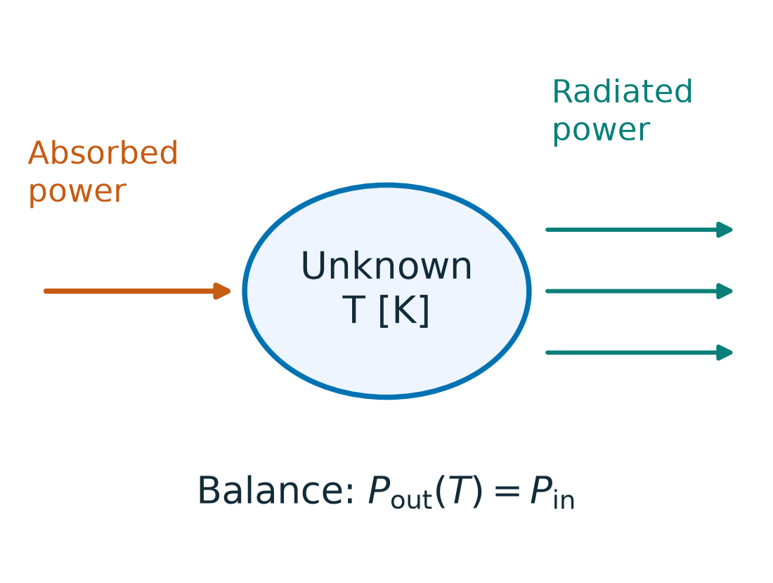
Find a physical balance¶

A body absorbs power and radiates into a cold environment. Which temperature balances the two?

f(T)=P_{\rm out}(T)-P_{\rm in}=0.

(1)

An event time is similar: when does position minus a boundary become zero?

The unknown is an input to a model we can evaluate.

Incoming power heats a body; emitted power depends on its unknown temperature. — Powers use erg/s; temperature uses kelvin.

Why this matters · invert a relationship in data science¶

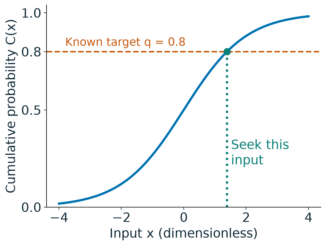
Find a probability threshold¶

Given a probability $q$ , seek $x$ with $C(x)-q=0$ .

Here $C$ is a continuous, strictly increasing cumulative distribution function (CDF) and the bracket spans $q$ . Discrete CDFs need a generalized quantile definition.

ML/AI: stationary conditions and implicit models also define outputs through equations. A stationary point need not be a minimum.

A continuous cumulative probability curve crosses the target probability at a threshold input. — Known: target probability. Unknown: its input threshold.

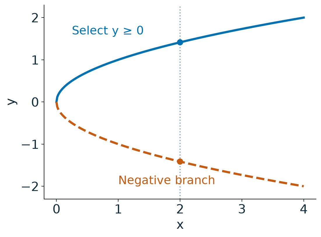
Explicit and implicit describe how we state a relation¶

y=\sqrt{x}\quad\hbox{versus}\quad y^2-x=0.

(2)

For $x>0$ , the implicit relation includes two branches. Requiring $y\ge0$ selects the square root.

Implicit does not mean impossible to rearrange. More elaborate models can require numerical inversion.

Taylor approximation already supplied quadrature and slopes. We now use those ideas to make numerical decisions.

Both positive and negative square-root branches satisfy the implicit relation.

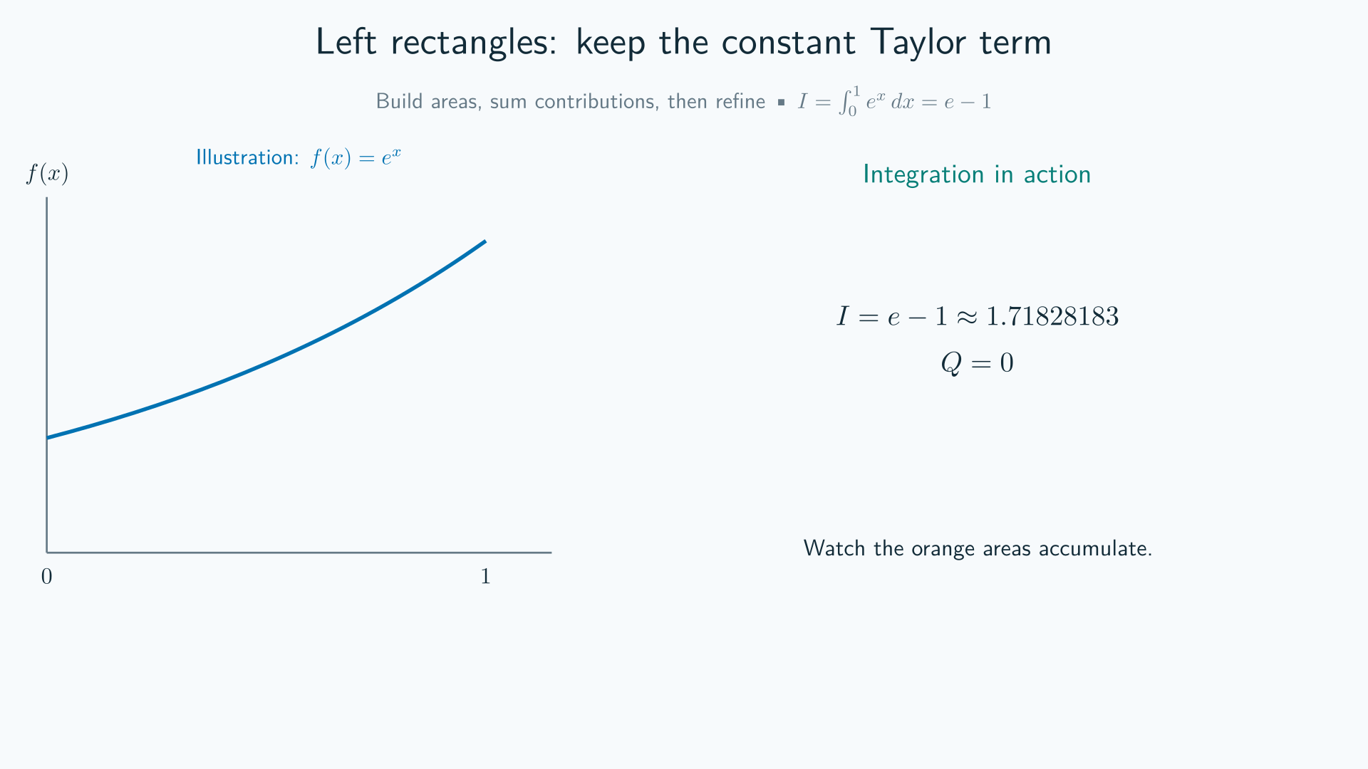
Recall · left rectangles from Taylor¶

Left rectangles accumulate across the interval, then refine from four to eight to sixteen panels with running sums and actual error; Taylor explains local second-order and composite first-order truncation error.

Open or download this short animation

Video page and explanation

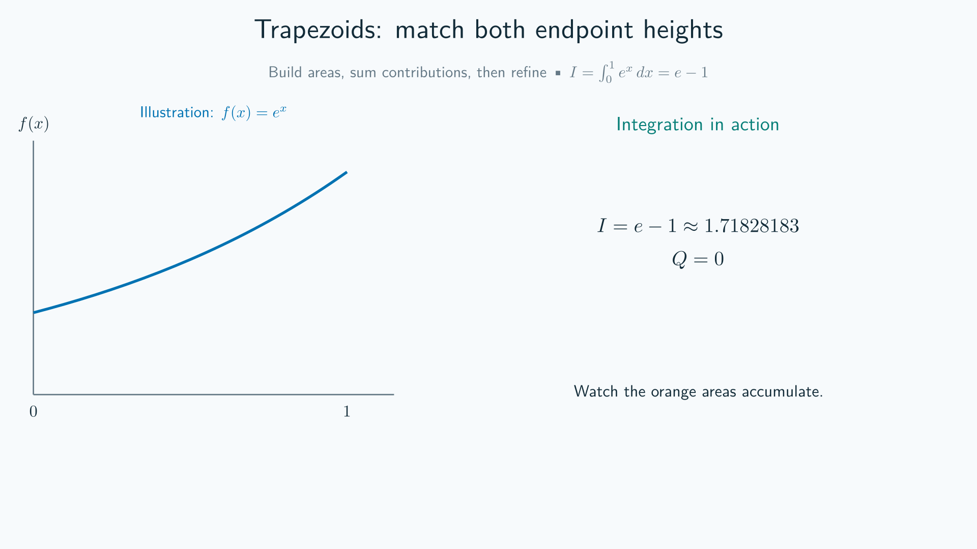
Integration in action, then Taylor recall. Interpret: why does an error of order $h^2$ on one panel give order $h$ over a fixed interval?

Recall · trapezoids from Taylor¶

Trapezoidal areas accumulate and the partition refines, with running sums and actual error; comparing Taylor coefficients gives local third-order and composite second-order truncation error.

Open or download this short animation

Video page and explanation

Integration in action, then Taylor recall. Interpret: which Taylor terms agree, and which coefficient first differs?

Recall · Simpson from Taylor and symmetry¶

Quadratic segments accumulate their areas across successive Simpson pairs; refinement changes the sum and actual error, then Taylor symmetry explains fifth-order pair error and fourth-order composite error.

Open or download this short animation

Video page and explanation

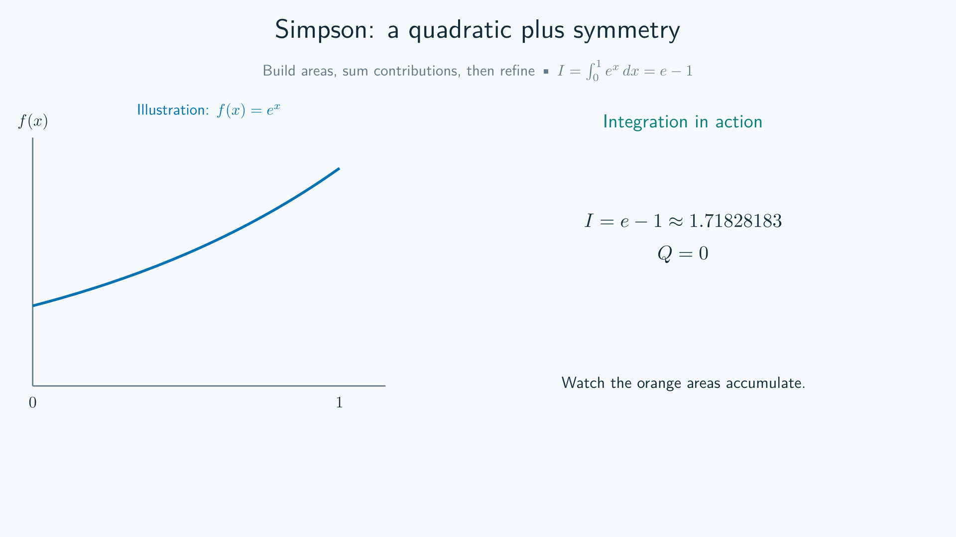
Integration in action, then Taylor recall. Interpret: why is a rule built from a quadratic also exact for cubics? The pair width is $2h$ .

I · Adaptivity uses an error estimate to allocate work¶

Question: where does another function evaluation help most?

Recall Simpson’s fourth-order composite error for sufficiently smooth functions.
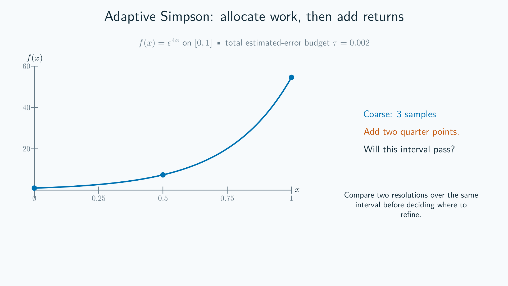
Compare coarse and fine estimates on the same interval.
Refine intervals whose estimated error exceeds their budget.

Uniform refinement doubles work everywhere. Adaptive refinement concentrates work where the current estimate indicates it is needed.

Estimate an integral error without knowing the integral¶

Here $I$ is the unknown integral, $h$ is the grid spacing, and $p$ is the method’s error order. $C$ is the leading error coefficient, independent of $h$ . For a fixed interval, suppose a leading error term dominates:

Q(h)=I+Ch^p+\cdots.

(3)

Refine the grid:

Q(h/2)=I+\frac{Ch^p}{2^p}+\cdots.

(4)

Question: subtract the two expressions. Which unknown disappears?

Richardson: cancel the unknown integral¶

Subtract:

Q(h/2)-Q(h)\approx Ch^p(2^{-p}-1).

(5)

Solve for the correction to the finer estimate:

I-Q(h/2)\approx\frac{Q(h/2)-Q(h)}{2^p-1}.

(6)

The difference estimates what the finer grid still misses. The factor $2^p-1$ converts a change between grids into an estimated fine-grid error.

This needs a dominant leading error term; agreement alone is not a guarantee.

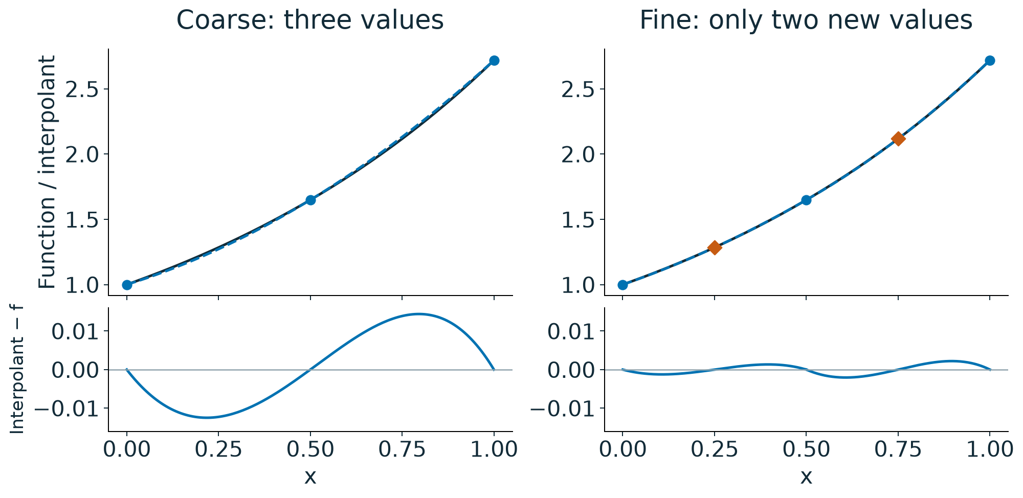
Coarse and fine reuse the same samples¶

One quadratic uses three blue samples; two half-interval quadratics reuse these and add two orange diamond samples. — For $f(x)=e^x$ on $[0,1]$ , both estimates cover the same interval. Dashed curves are quadratic interpolants; the lower panels show their pointwise errors on the same scale.

Write the estimates from the picture¶

Let $m=(a+b)/2$ . A Simpson pair has width $H=b-a=2h$ , where $h$ is Lecture 6’s elementary-panel width.

S=\frac{H}{6}\,[f(a)+4f(m)+f(b)].

(7)

Apply Simpson on each half and add:

S_2=S_{[a,m]}+S_{[m,b]}.

(8)

Each half has its own midpoint. The three old samples are reused; only two additional function evaluations are needed.

The leading error of one Simpson pair scales as $H^5$ for a sufficiently smooth function. Its signed error is $I-S=-H^5f^{(4)}(\xi)/2880$ for some $\xi\in(a,b)$ when the fourth derivative is continuous.

Two half-width pairs contribute, to leading order,

2\left(\frac{H}{2}\right)^5=\frac{H^5}{16}.

(9)

This assumes the leading local error coefficient is approximately shared across the interval.

Thus $S_2$ has about $1/16$ of the leading error of $S$ . Their difference is about 15 times the remaining error in $S_2$ .

Simpson gives the factor 15¶

Let $S$ use one Simpson pair, and $S_2$ use its two halves.

e_{\rm est}=\frac{|S_2-S|}{2^4-1}=\frac{|S_2-S|}{15}.

(10)

The corrected estimate is

S_{\rm corrected}=S_2+\frac{S_2-S}{15}.

(11)

The estimator describes the uncorrected fine result $S_2$ . It is not a proven bound on the corrected result’s error.

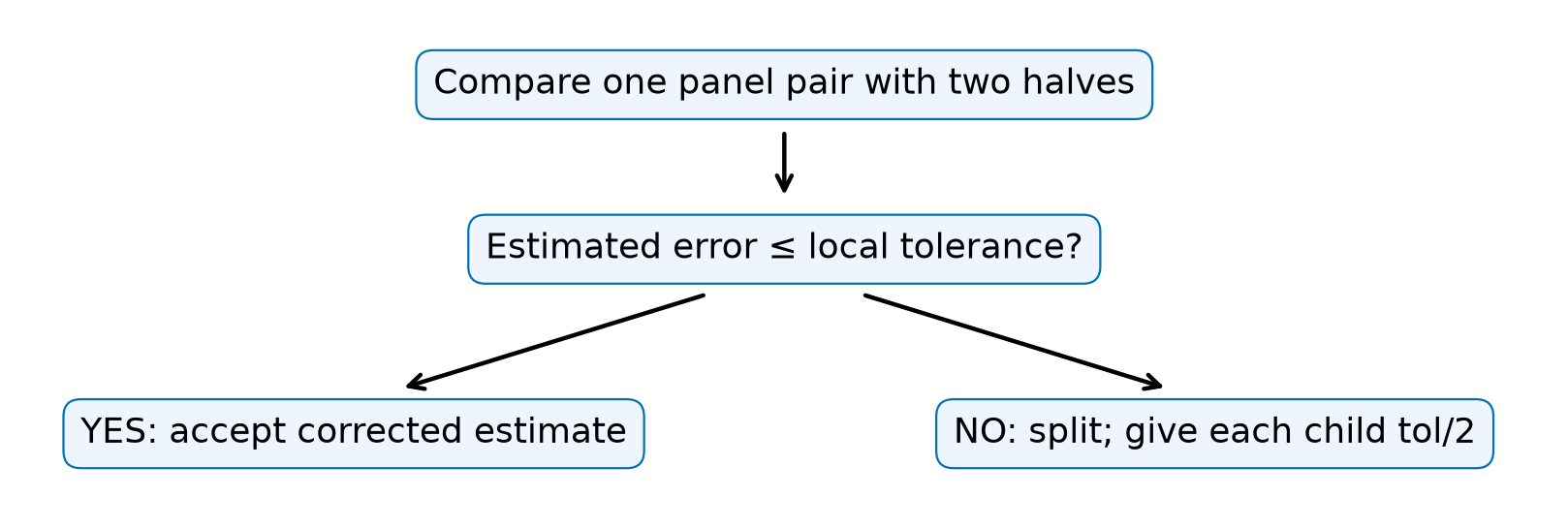
Predict: accept this interval or subdivide?¶

An illustrative calculation gives

S=1.20000,\qquad S_2=1.20030,\qquad \tau=10^{-5}.

(12)

Calculate $|S_2-S|/15$ .
Compare it with the local tolerance $\tau$ .
What should the algorithm do next?

e_{\rm est}=\frac{0.00030}{15}=2\times10^{-5}>\tau.

(13)

Subdivide. Give each child a local tolerance of $\tau/2$ .

The child budgets add to the parent’s budget. Accepted estimated errors can be budgeted this way; they are not unconditional bounds on the true error.

Optional live experiment: compare the estimator with actual error.

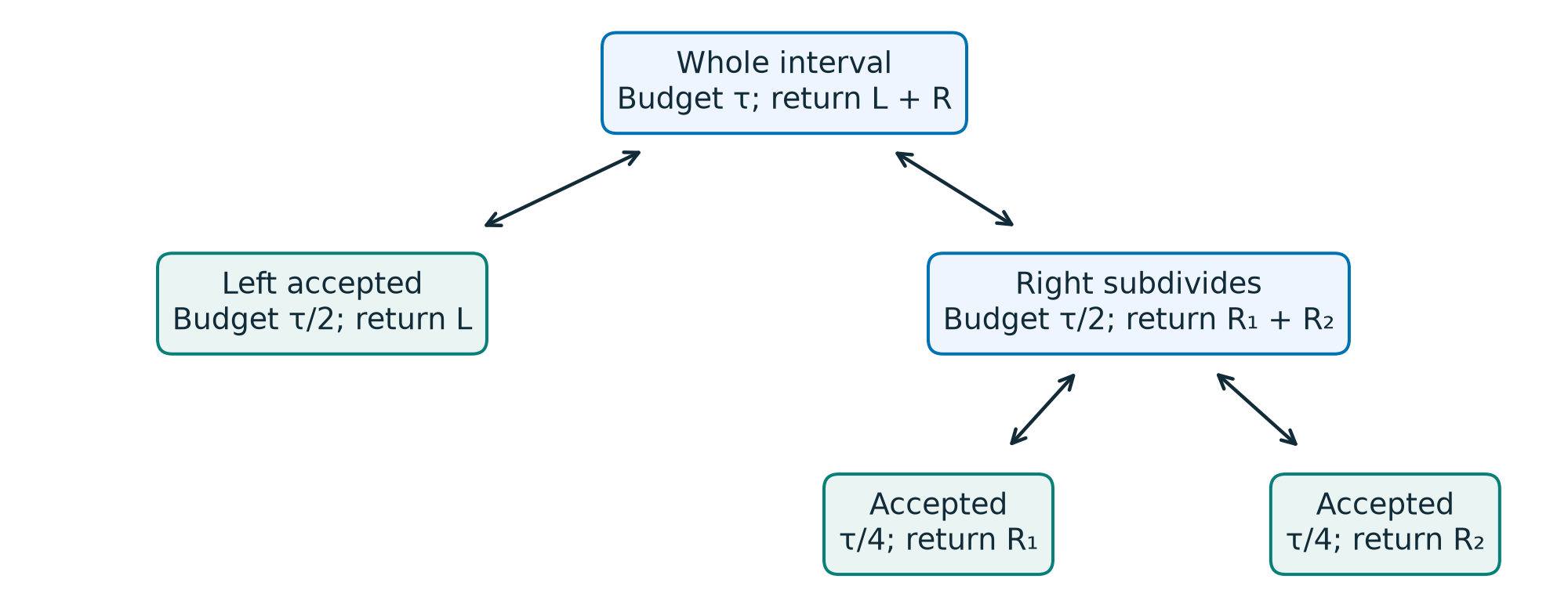
Pass budgets down; add integral estimates back up¶

A parent delegates two half budgets; accepted leaves return contributions that are added by their parents. — A leaf accepts and returns a corrected integral estimate. A parent adds its children’s returns. The accepted budgets sum to the original tolerance.

This is recursion: repeat the task on smaller intervals and combine their returns. Optional animated example.

Watch · adaptive quadrature allocates work¶

Adaptive Simpson fills coarse and refined quadratic areas, splits local budgets, and accumulates accepted corrected contributions with covered-interval actual error.

Open or download this short animation

Video page and explanation

Integration in action. Interpret: what travels down the recursion tree, and what comes back up? The error estimate is not an unconditional bound.

Reuse samples; do not hide failure¶

Reuse¶

A parent has values at $a$ , $m$ , and $b$ .

Its two halves need only two new quarter-point values. Pass the existing values down.

Stop honestly¶

Invalid tolerance or depth: reject the input.
Estimate meets tolerance: accept the corrected value.
More refinement needed, depth exhausted: raise RuntimeError.

Do not return an unfinished sum as success.

Agreement can miss unsampled structure¶

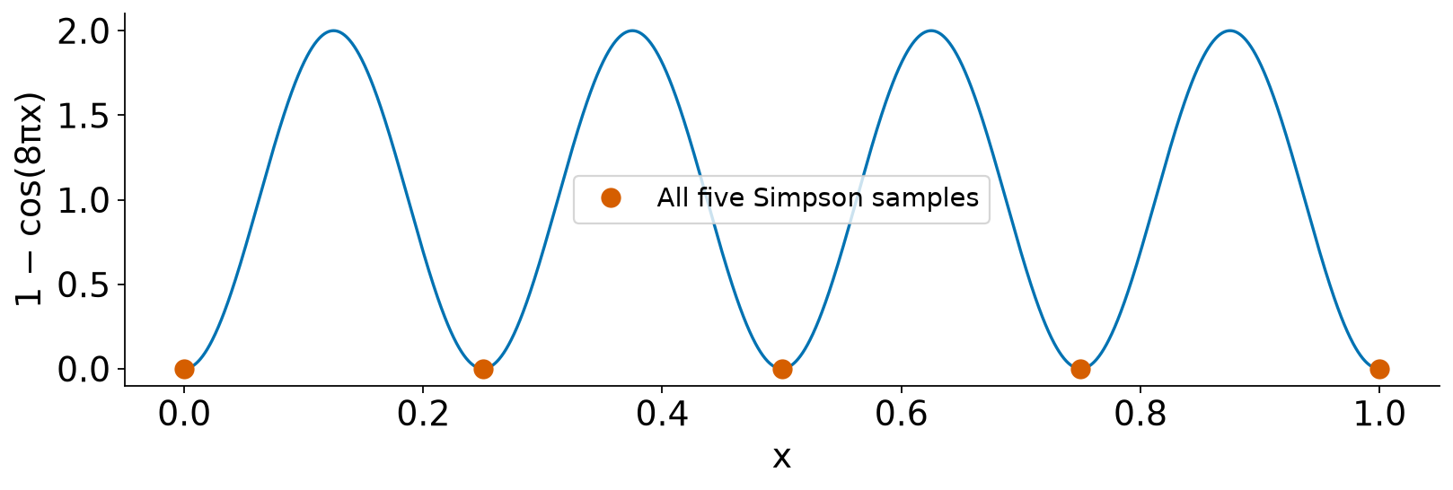
The oscillating function has four humps, but all five sampled positions have value zero. — For $f(x)=1-\cos(8\pi x)$ on $[0,1]$ , both estimates are approximately zero; the exact integral is 1. This is twice the reading’s $\sin^2(4\pi x)$ example.

What the missed wave teaches us¶

At $x=0,1/4,1/2,3/4,1$ , the cosine equals 1, so every sampled height vanishes.

But

\int_0^1[1-\cos(8\pi x)]\,dx =\left[x-\frac{\sin(8\pi x)}{8\pi}\right]_0^1=1.

(14)

The estimator cannot detect structure absent from its samples. Use known oscillation scales or breakpoints to guide sampling, and compare independent refinements.

Explain: would tightening the tolerance change an exactly zero estimated error?

II · Bisection preserves a statement we can trust¶

Question: can we narrow down an unknown input without using a derivative?

Find an interval whose endpoint values have opposite signs.
Use continuity to establish that at least one root lies inside.
Keep that statement true while shrinking the interval.

This preserved statement is the invariant. It connects the mathematical argument to the loop you will later write.

Change the task: locate a zero¶

Our shared example is

f(x)=x^2-2,\qquad x\in[1,2].

(15)

The positive root is $r=\sqrt{2}$ , an independent check for this teaching example.

$x$ : our current estimate of the root.
$f(x)$ : the residual.
$|x-r|$ : the root error, available here because we know $r$ .

A bracket gives a guarantee¶

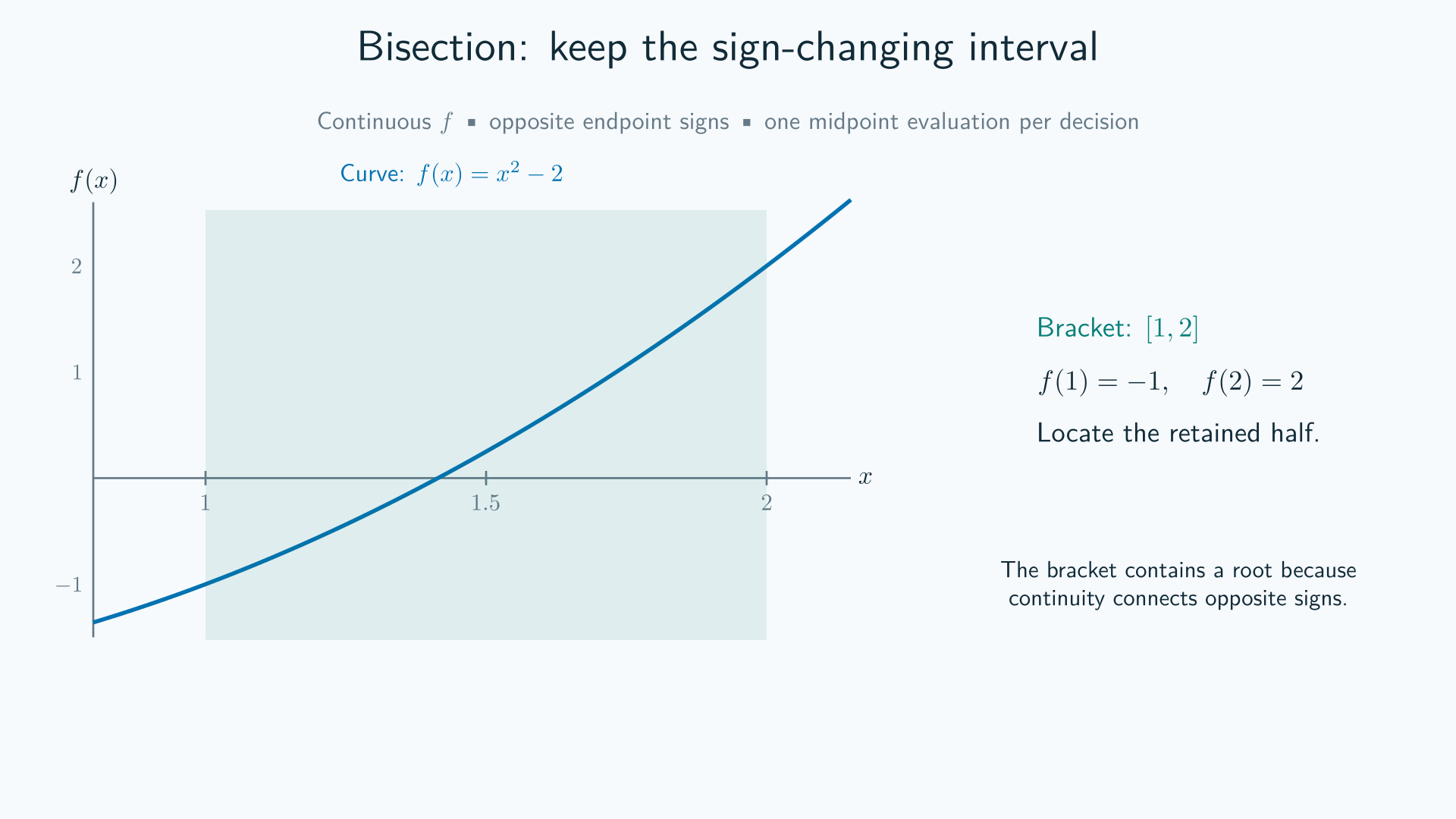
For continuous $f$ on $[a,b]$ , opposite endpoint signs imply at least one root inside.

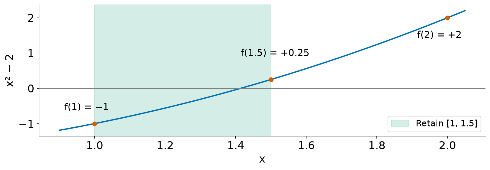
Here $f(1)=-1$ and $f(2)=2$ .

Predict: the midpoint is $m=1.5$ . Which half should we retain?

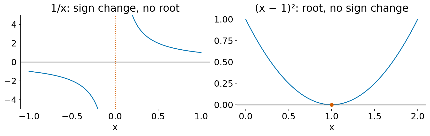
Check endpoint roots before requiring opposite signs. A sign change across a discontinuity is not this theorem.

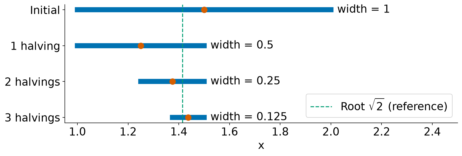
Watch the bracket shrink¶

Three bisection decisions preserve opposite signs and halve the interval width.

Open or download this short animation

Video page and explanation

Interpret: the bound after an update belongs to the new bracket’s midpoint. It does not apply to the old midpoint.

Static companion

A sign change needs continuity¶

One over x changes sign across a discontinuity without a root; a squared function touches zero without changing sign. — Left: the continuity hypothesis fails. Right: a root can exist without opposite endpoint signs.

Existence is different from uniqueness¶

For a continuous function, opposite endpoint signs guarantee at least one root.

They do not establish that there is only one.

For our example on $[1,2]$ ,

f'(x)=2x>0.

(16)

Strict increase rules out two distinct roots in this interval. We know which root the shrinking brackets locate.

Each halving reduces the uncertainty¶

Four nested brackets shrink toward square root of two, with orange midpoint markers and the width of each interval shown. — The bracket is the evidence. Its midpoint need not have the smallest residual among all points already sampled.

The bracket gives a root-error bound¶

The root lies somewhere inside the retained interval. The midpoint is at most half its width from any point in that interval:

|m-r|\le\frac{b-a}{2}.

(17)

This bounds root location, even though the exact root is unknown.

The residual $f(m)$ measures a different quantity: how well the equation is satisfied.

How many halvings meet the target?¶

After $k$ halvings of an initial width $W_0$ ,

W_k=\frac{W_0}{2^k},\qquad |m_k-r|\le\frac{W_0}{2^{k+1}}.

(18)

For $W_0=1$ and an absolute target 10^-3:

2^{-10}\approx0.000977<0.001.

(19)

Nine halvings suffice for the midpoint of the resulting interval. Evaluating it is the tenth midpoint evaluation, counting the initial midpoint first; distinguish halvings from function evaluations.

III · Newton uses the local slope¶

Question: can local shape suggest a larger, more useful step?

Bisection uses signs and interval width. Newton uses a value and a derivative.

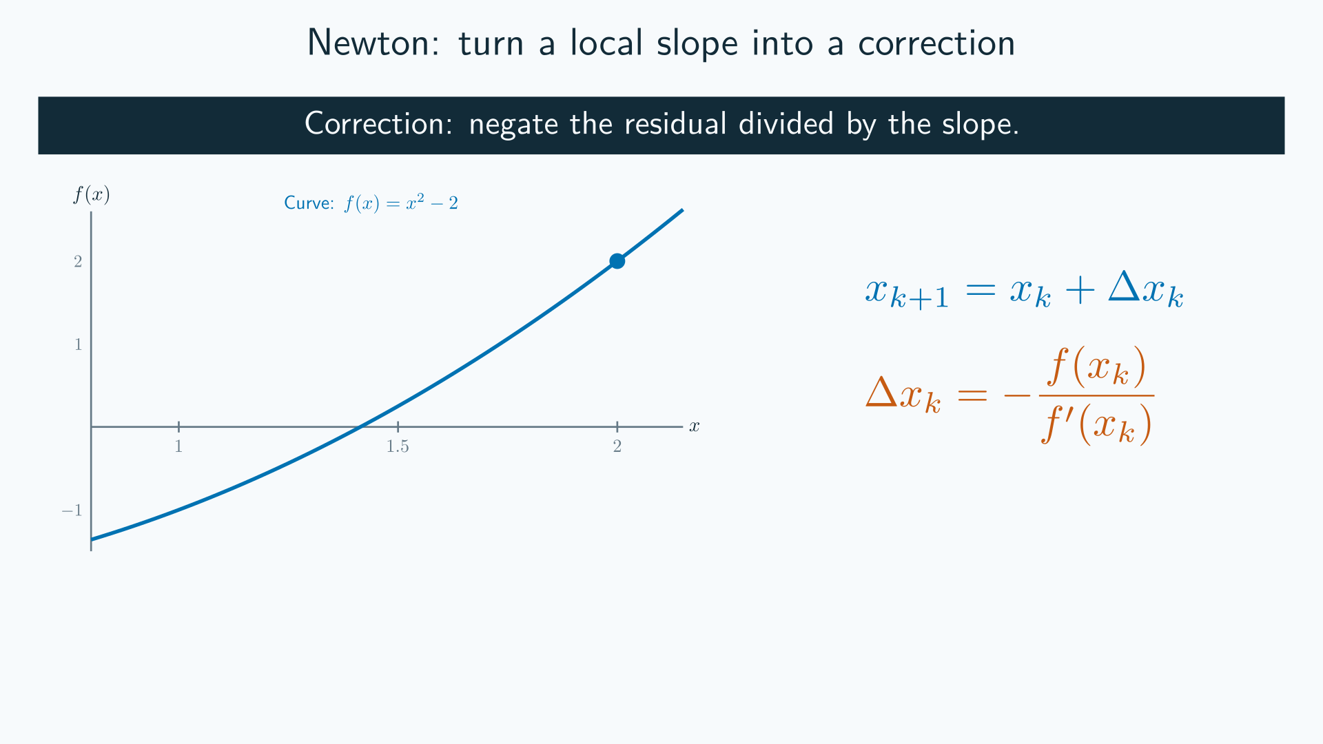
Replace the curve by its tangent near the current point.
Find the tangent’s zero.
Rebuild the tangent at the new point.

The same Taylor approximation that explained quadrature errors now supplies an update rule.

Newton solves a Taylor approximation¶

Near the current estimate $x_k$ ,

f(x_k+\Delta x)\approx f(x_k)+f'(x_k)\Delta x.

(20)

Set the linear model to zero:

\Delta x=-\frac{f(x_k)}{f'(x_k)},\qquad x_{k+1}=x_k-\frac{f(x_k)}{f'(x_k)}.

(21)

We solve the local model exactly; the model itself is approximate.

Predict the tangent step¶

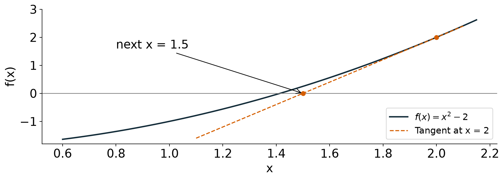
For $f(x)=x^2-2$ , $f'(x)=2x$ .

Start at $x_0=2$ :

x_1=2-\frac{2^2-2}{2(2)}.

(22)

Calculate the next iterate. Does it move toward the positive root?

Watch the tangent, then return to the curve¶

Newton takes two updates from two: construct a tangent, find its zero, then reevaluate the original curve.

Open or download this short animation

Video page and explanation

Interpret: why must we return to the curve before building the next tangent?

First tangent · Second tangent zoom

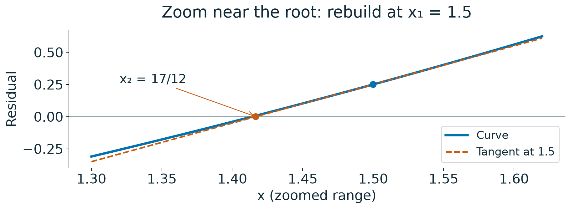
Rebuild the tangent at the new point¶

A zoomed curve and new tangent at one point five give the next iterate seventeen twelfths. — At $x_1=1.5$ , the slope is now 3. The new tangent gives $x_2=1.5-0.25/3=1.416667\ldots$ .

Why Newton needs another local model¶

The previous tangent matched the curve at the previous point. Moving changes both the function value and its slope.

Each iteration therefore:

evaluates the remaining residual;
builds a new tangent; and
uses that tangent’s zero as the next estimate.

The index $k$ counts updates, not time steps. A simple root satisfies $f(r)=0$ and $f'(r)\ne0$ . Sufficient smoothness and a sufficiently close starting point can give rapid convergence.

Run: connect each update to the geometry¶

Each row below describes the new iterate after an update. The step is signed; the residual is evaluated at that new iterate.

# lecture-example: newton
x = 2.0
print(" k       x_new       step       f(x_new)")
for k in range(1, 4):
    step = -(x*x - 2) / (2*x)
    x = x + step
    print(f"{k:2d}  {x:.8f}  {step:+.3e}  {x*x-2:+.3e}")

Interpret after running: which columns describe movement and which describe satisfaction of the equation?

Prepared output. This calculation is specific to $x^2-2$ ; students build general solvers later.

Prepared output: Newton updates¶

Update	New iterate	Signed step	Residual at new iterate
1	1.50000000	−5.000e−1	+2.500e−1
2	1.41666667	−8.333e−2	+6.944e−3
3	1.41421569	−2.451e−3	+6.007e−6

The residual decreases in this example. These three rows do not establish convergence from every initial guess.

Explain: which operation in the code corresponds to returning from the line to the curve?

When the tangent is a poor guide¶

Example: $x^2-2$ ¶

At $x=0$ , the derivative is zero: the update is undefined.

Near zero, dividing by a small slope can produce a very large step.

What matters¶

The starting point.
Whether the derivative is usable.
Whether the next point remains in the domain.

A fast local method does not automatically preserve a bracket.

IV · Project 2 continuation¶

If time remains, discuss Project 2 questions together, then continue your work.

Continue your quadrature implementations and tests.
Check convergence against the assumptions behind each rule.
Bring a failing test, unexpected plot, or unresolved design question.

If blocked: show the smallest reproducible case and what you expected.

No root-finding activity in this work block.

V · Reference and optional demonstrations¶

The teaching path ends after Newton, followed by Project 2 discussion and work if time remains. These derivations, static companions, and optional demonstrations remain available for review.

The teaching budget includes the recall and method animations. These additional reference demonstrations are available for independent review.

Today’s question¶

How can an approximation tell us where to spend work—and which input to try next?

By the end of class, you should be able to:

explain the coarse–fine error estimate behind adaptive Simpson;
turn an implicit relation into a residual;
trace bisection and justify its root-error bound; and
derive Newton’s update from a first-order Taylor model.

Plan: about 70 minutes: 5 min motivation · 10 min quadrature recall · 25 min adaptivity · 12 min bisection · 18 min Newton. Any remaining class time is for Project 2 questions and continuation.

The relation contains both branches¶

Positive and negative square-root branches with two intersections at x equals two. — Fixing $x=2$ leaves two possible values of $y$ . Requiring $y\ge0$ selects one branch.

Implicit does not mean impossible to rearrange¶

Here, algebra isolates $y$ . Other relations resist a useful explicit formula.

For a fixed parameter $x$ , define a residual:

F(y)=y^2-x.

(23)

Root finding asks for an input $y$ that makes $F(y)=0$ .

Later: an implicit ODE step contains the unknown future state and can require a solve.

Start with a physical balance¶

A toy body receives constant power $P_{\rm in}$ and radiates into a cold environment:

P_{\rm out}(T)=\epsilon\sigma A T^4.

(24)

$T$ : absolute temperature in kelvin; $A$ : surface area.
$\epsilon$ : emissivity; $\sigma$ : Stefan–Boltzmann constant.
Both $P_{\rm in}$ and $P_{\rm out}$ are powers, measured in erg/s with consistent CGS constants.

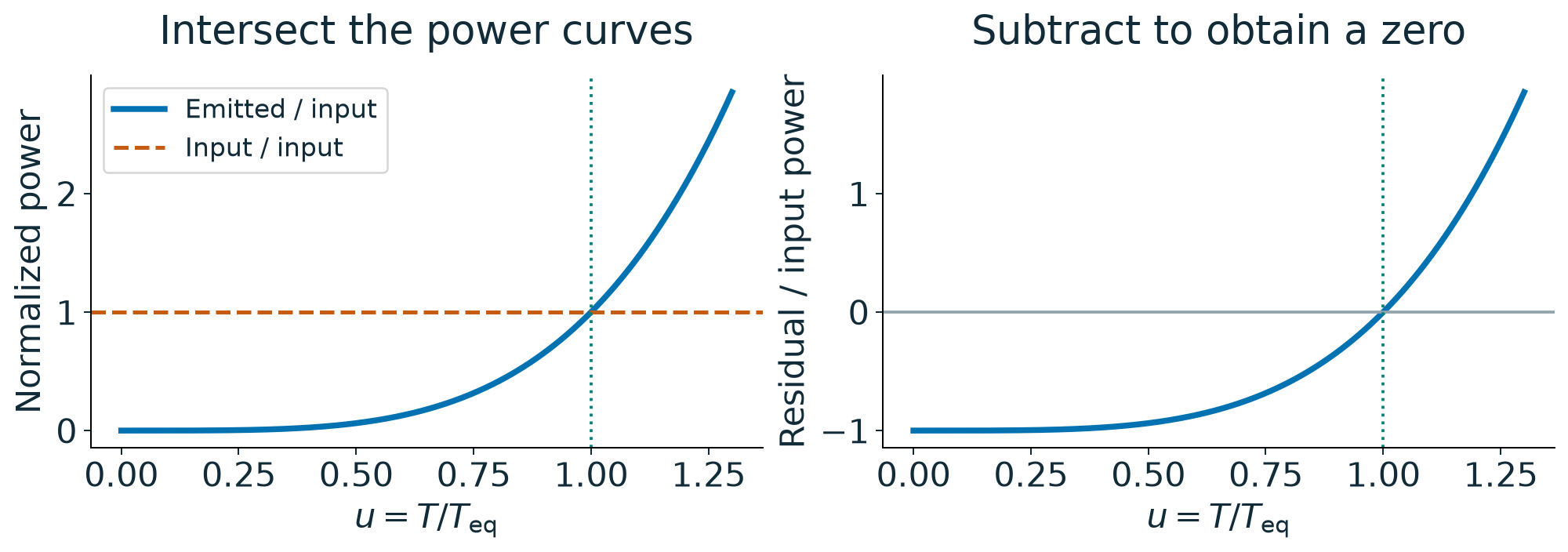
Question: what equation expresses thermal balance?

Turn an intersection into a zero¶

Left panel shows input and emitted powers intersecting; right panel shows their difference crossing zero at the same temperature. — $F(T)=P_{\rm out}(T)-P_{\rm in}=0.$
(25)

The dimensionless plot uses $u=T/T_{\rm eq}$ , where $T_{\rm eq}$ is the illustrative equilibrium reference. This constant-emissivity model has an explicit answer. Temperature-dependent properties can require a numerical solve. A root establishes balance, not stability.

Watch the adaptive decisions¶

For exp(4x), compare coarse and fine Simpson estimates, allocate half budgets on a split, and add accepted contributions.

Open or download this short animation

Video page and explanation

Interpret: why does the right half need more samples? This is estimator-guided allocation, not a universal guarantee. Return to sample reuse.

Static companion: the adaptive decision¶

Compare the error estimate with the tolerance; accept a corrected estimate or subdivide. — The split branch requires remaining refinement depth; otherwise report failure.

Adaptive integration summary¶

Quantity	Meaning
$S_2-S$	Difference between two resolutions
$\vert S_2-S\vert /15$	Estimated fine-grid Simpson error
$S_2+(S_2-S)/15$	Corrected estimate
Child budgets $\tau/2$	Equal allocation of the parent’s tolerance
Depth limit	A failure guard, not evidence of accuracy

Reading: adaptive quadrature and Richardson.

Static frame: keep opposite signs¶

The retained interval is one to one point five; its endpoint signs are opposite. — $f(1.5)=0.25>0$ , so retain $[1,1.5]$ .

Static frame: Newton’s first tangent¶

The tangent at two crosses at one point five, distinct from the curve’s root.

Brackets and local models¶

Method	Information	What the step preserves
Bisection	Continuous function and sign-changing bracket	A bracket containing a root
Newton	Function, derivative, starting point	No bracket guarantee by itself

A small step, a small residual, and a small root error are different claims.

Reading: root-finding geometry and methods.

Run: does the Simpson estimate track the error?¶

For $e^x$ on $[0,1]$ , the reference integral is $e-1$ . Predict the change in error when the spacing halves.

# lecture-example: simpson
import numpy as np
x = np.linspace(0.0, 1.0, 5)
y = np.exp(x)
coarse = (y[0] + 4*y[2] + y[4]) / 6
fine = (y[0] + 4*y[1] + 2*y[2] + 4*y[3] + y[4]) / 12
correction = (fine - coarse) / 15
exact = np.expm1(1.0)
print("fine error:", abs(fine - exact))
print("estimate:  ", abs(correction))
print("corrected: ", abs(fine + correction - exact))

Interpret the differences; the exact reference lets us test an estimator. This is one fixed sample calculation, not an adaptive implementation.

Prepared output: Simpson comparison¶

Quantity	Approximate magnitude
Fine Simpson error	3.70e−5
Estimated fine error	3.62e−5
Corrected-result error	8.59e−7

The estimator is close in this smooth example. The corrected result is more accurate here, but the estimate is neither its measured error nor a rigorous bound.

Lecture 7 · Approximations, Adaptivity, and Roots

From a local model to a numerical decision¶

Why this matters · infer an input in computational science¶

Find a physical balance¶

Why this matters · invert a relationship in data science¶

Find a probability threshold¶

Explicit and implicit describe how we state a relation¶

Recall · left rectangles from Taylor¶

Recall · trapezoids from Taylor¶

Recall · Simpson from Taylor and symmetry¶

I · Adaptivity uses an error estimate to allocate work¶

Estimate an integral error without knowing the integral¶

Richardson: cancel the unknown integral¶

Coarse and fine reuse the same samples¶

Write the estimates from the picture¶

Why refinement gives a factor of 16¶

Simpson gives the factor 15¶

Predict: accept this interval or subdivide?¶

Decision: subdivide and share the budget¶

Pass budgets down; add integral estimates back up¶

Watch · adaptive quadrature allocates work¶

Reuse samples; do not hide failure¶

Reuse¶

Stop honestly¶

Agreement can miss unsampled structure¶

What the missed wave teaches us¶

II · Bisection preserves a statement we can trust¶

Change the task: locate a zero¶

A bracket gives a guarantee¶

Watch the bracket shrink¶

A sign change needs continuity¶

Existence is different from uniqueness¶

Each halving reduces the uncertainty¶

The bracket gives a root-error bound¶

How many halvings meet the target?¶

III · Newton uses the local slope¶

Newton solves a Taylor approximation¶

Predict the tangent step¶

Watch the tangent, then return to the curve¶

Rebuild the tangent at the new point¶

Why Newton needs another local model¶

Run: connect each update to the geometry¶

Prepared output: Newton updates¶

When the tangent is a poor guide¶

Example: x2−2x^2-2x2−2¶

What matters¶

IV · Project 2 continuation¶

V · Reference and optional demonstrations¶

Today’s question¶

The relation contains both branches¶

Implicit does not mean impossible to rearrange¶

Start with a physical balance¶

Turn an intersection into a zero¶

Watch the adaptive decisions¶

Static companion: the adaptive decision¶

Adaptive integration summary¶

Static frame: keep opposite signs¶

Static frame: Newton’s first tangent¶

Brackets and local models¶

Run: does the Simpson estimate track the error?¶

Prepared output: Simpson comparison¶

Example: $x^2-2$ ¶