Animation · Newton's method - COMP 521: Introduction to Scientific Computing and Data Science

Starting at $x_0=2$ for $f(x)=x^2-2$ , replace the curve locally by its tangent, find the tangent’s zero, and return to the original curve. The film shows two updates.

Before watching¶

The first tangent starts at $(2,2)$ and has slope 4. Predict its horizontal displacement to the axis. After moving, can the same tangent supply the next update?

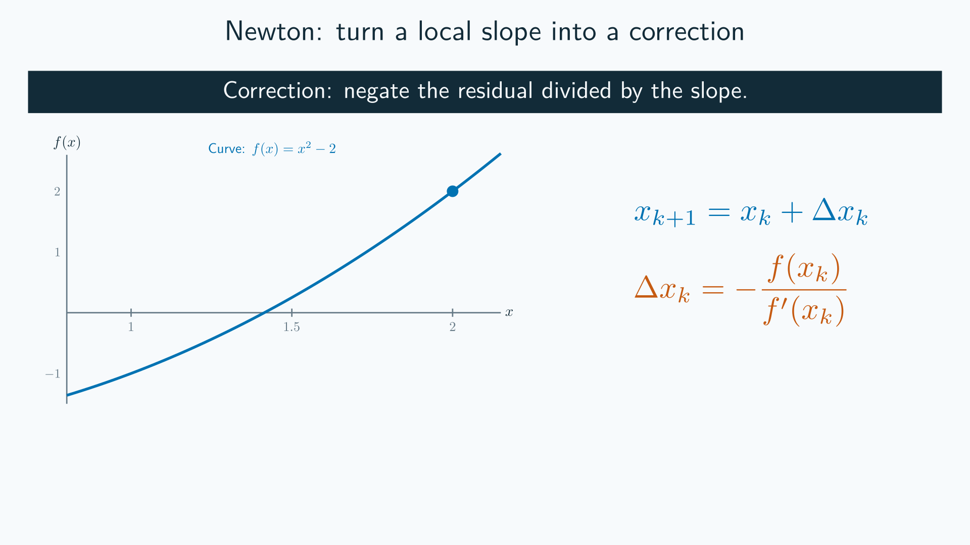
Starting at x_0=2 for f(x)=x^2-2, replace the curve locally by its tangent, find the tangent's zero, and return to the original curve. The film shows two updates.

Open or download this short animation

Mathematical connection¶

The first-order Taylor model near $x_k$ is

f(x_k+\Delta x)\approx f(x_k)+f'(x_k)\Delta x.

(1)

Set this model to zero and solve:

x_{k+1}=x_k-\frac{f(x_k)}{f'(x_k)}.

(2)

The model is approximate, even though its zero is calculated exactly in real arithmetic. The derivative must be nonzero and the proposed point must remain in the function’s domain. Sufficient smoothness, a simple root, and a sufficiently close starting point give local quadratic convergence. Newton does not preserve a bracket by itself.

Static walkthrough: one Newton update¶

Predict before opening: at $x_0=2$ , $f(2)=2$ and $f'(2)=4$ . What signed correction makes the tangent model zero? Will the curve’s residual also vanish?

Worked explanation: model → correction → reevaluation

1. Build the tangent model¶

The tangent at two matches the curve value two and derivative four; the model equation is zero equals two plus four times the correction.

0=f(2)+f'(2)\Delta x_0=2+4\Delta x_0.

(3)

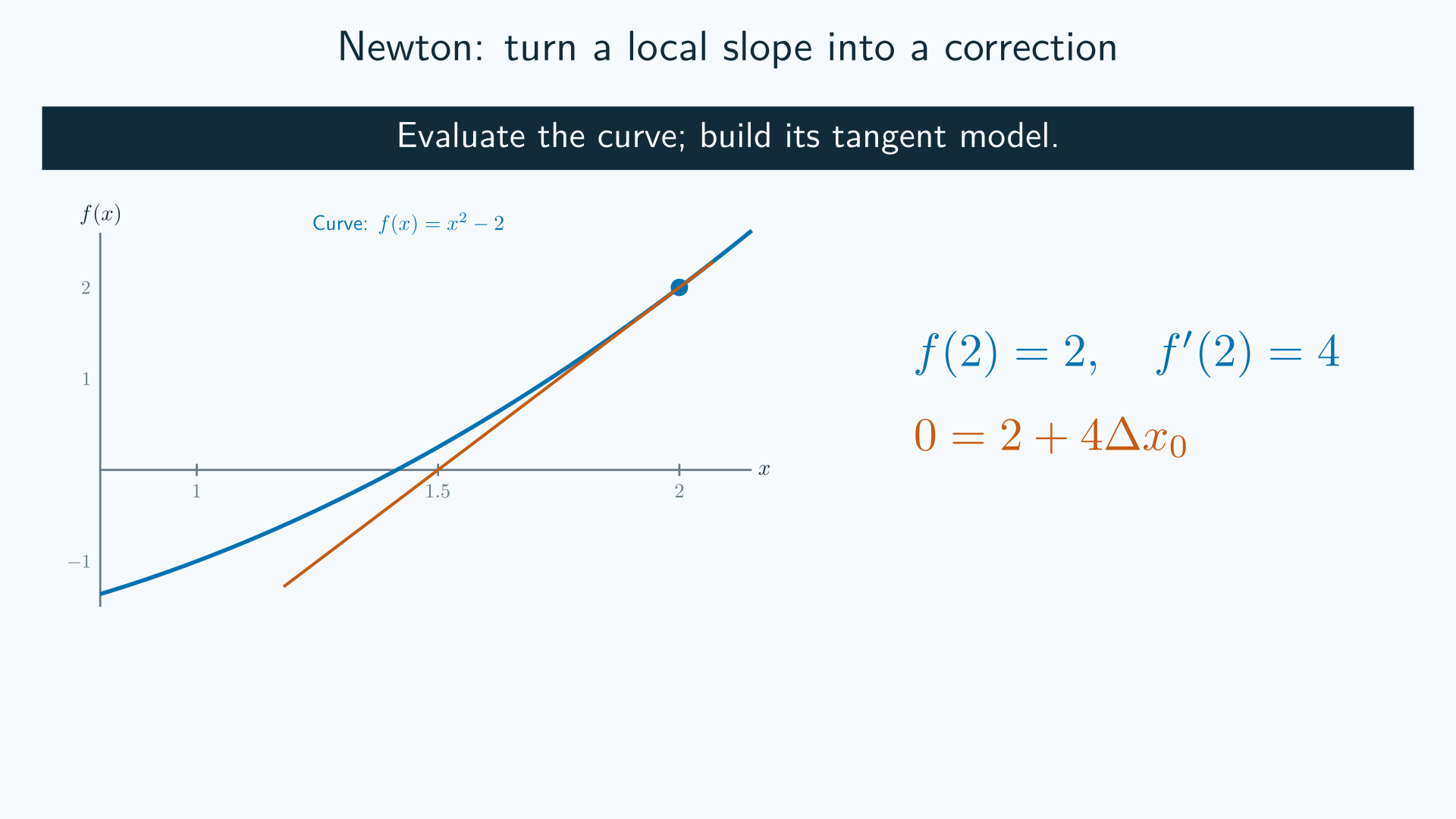
We set the linear model to zero; the original curve is only locally approximated.

2. Solve and move horizontally¶

A leftward arrow moves from two to three halves; the displayed correction is negative one half.

\Delta x_0=-\frac24=-\frac12,\qquad x_1=2-\frac12=\frac32.

(4)

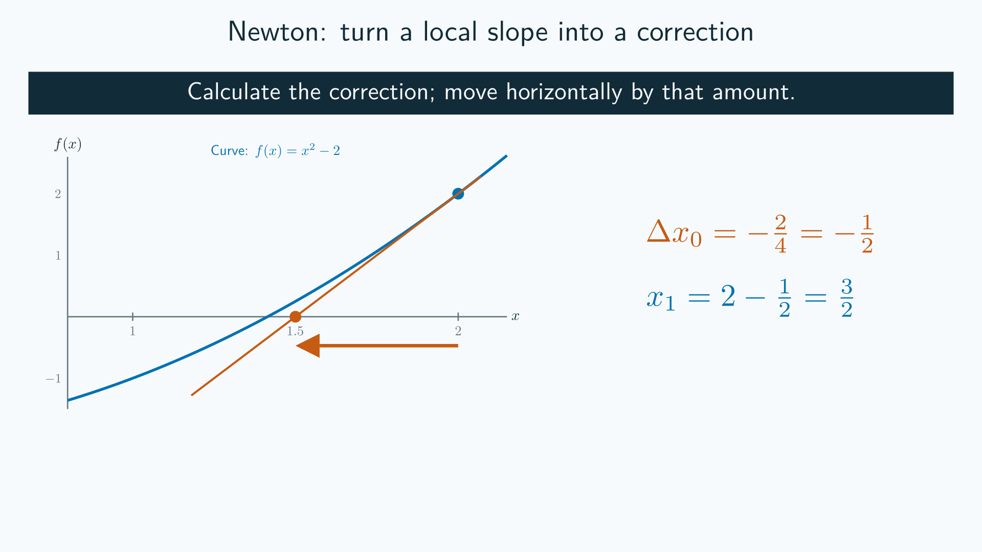
The negative correction moves the input left to the tangent’s zero.

3. Return to the curve¶

The new point is on the original curve at three halves with residual one quarter, above the tangent's zero.

f(3/2)=\frac94-2=\frac14,\qquad f'(3/2)=3.

(5)

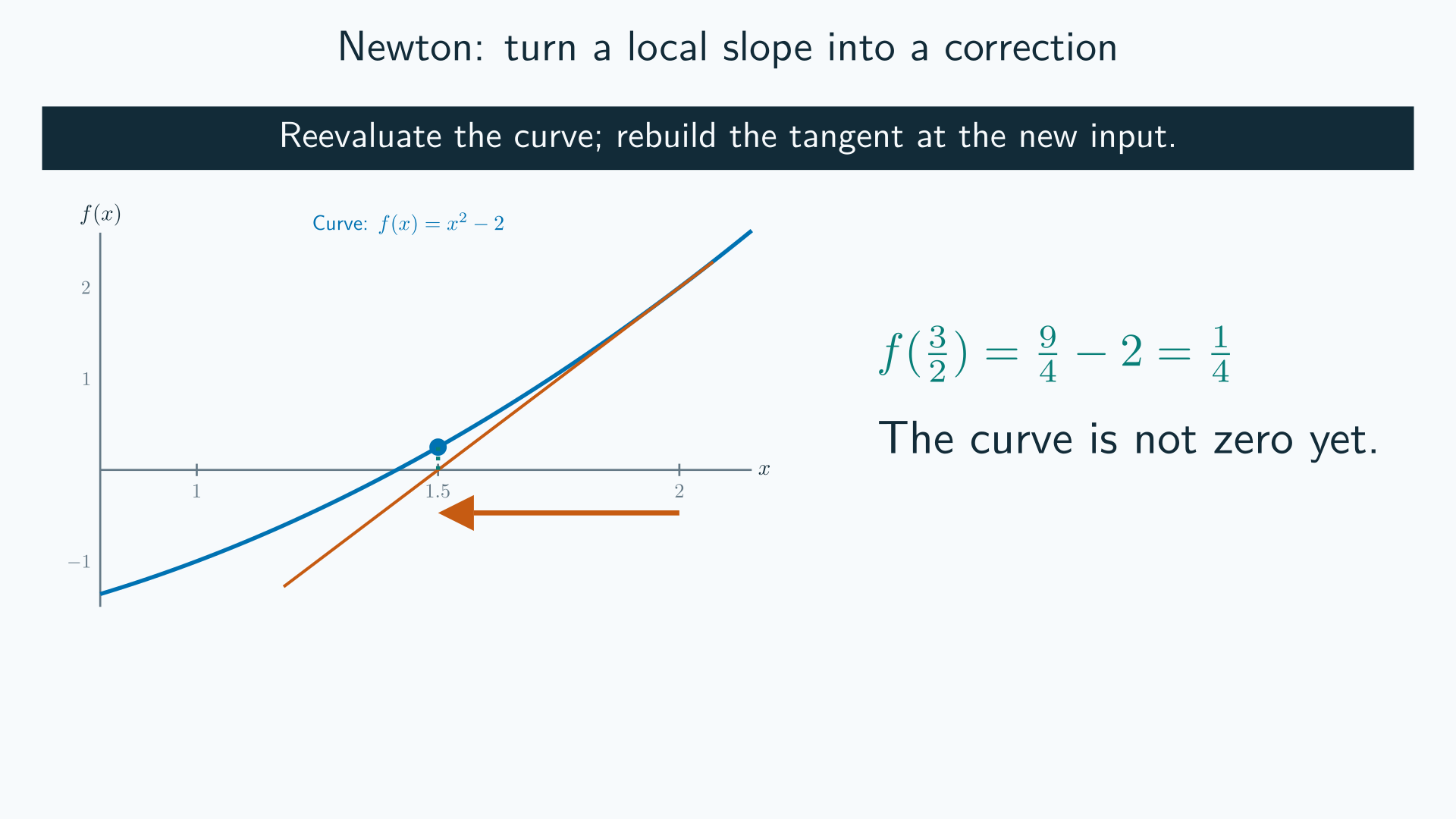
The residual is still nonzero. Recompute the slope and rebuild the tangent for the next update:

\Delta x_1=-\frac{1/4}{3}=-\frac1{12},\qquad x_2=\frac32-\frac1{12}=\frac{17}{12}.

(6)

The film’s second residual is $f(17/12)=1/144$ . A tangent’s zero is a proposed input, not an exact zero of the curve.

Explain what you saw¶

Find the moment when the animation returns from the axis to the curve. Explain why both the remaining residual and the tangent slope must be recomputed there.

Use the player controls to pause, replay, or view fullscreen. The animation has no narration. Burned-in captions explain each action; the static walkthrough above provides the same calculations without playback.

Continue: Lecture 7 · Full reading · All animations