Part 2: Floating-Point Arithmetic and Numerical Error
Module 1: Foundations of Discrete Computing | COMP 521
Mathematics treats real numbers as continuous and exact; computers store finite binary approximations. Numerical science begins when those worlds stop agreeing.
Learning Objectives
By the end of this section, you will be able to:
Compute for double precision and compare it with
np.finfo(float).eps.Distinguish representation error, truncation error, and accumulation or amplification error in scientific code.
Diagnose catastrophic cancellation and rewrite unstable expressions in algebraically equivalent, numerically safer forms.
Choose between and when comparing computed and true values.
Estimate how numerical error scales across astrophysical lengths, masses, times, and iterative update counts.
Use simple error-control and convergence-testing logic to decide whether a computation is trustworthy.
Why This Matters for Astronomy
Why this matters: astronomy forces us to compute across enormous ranges of scale, and floating-point arithmetic does not adapt its precision automatically to the physics we care about.
Student mental model: the computer does not store “the real number.” It stores the nearest representable binary value. That approximation is often excellent, but when we subtract nearly equal numbers, span many orders of magnitude, or iterate millions of times, the approximation can shape the science.
Astronomical simulations routinely cross very different physical scales:
Mercury orbits at , while Neptune orbits at .
A molecular cloud may span , while a protostellar core can be .
A star-forming region might be , while a galactic halo extends to .
If we work in CGS units, then these scales are
which says that even an inner-planet orbit already lives at trillions of centimeters.
which says that a solar-system calculation can span more than two orders of magnitude in position even before we consider velocities and forces.
which says that star-formation problems mix local structure and cloud-scale structure in the same calculation.
Double precision gives about 15 to 16 decimal digits of relative precision near numbers of order unity. That is an approximate practical statement about floating-point spacing, not a law of nature about “how many digits exist” in a calculation.
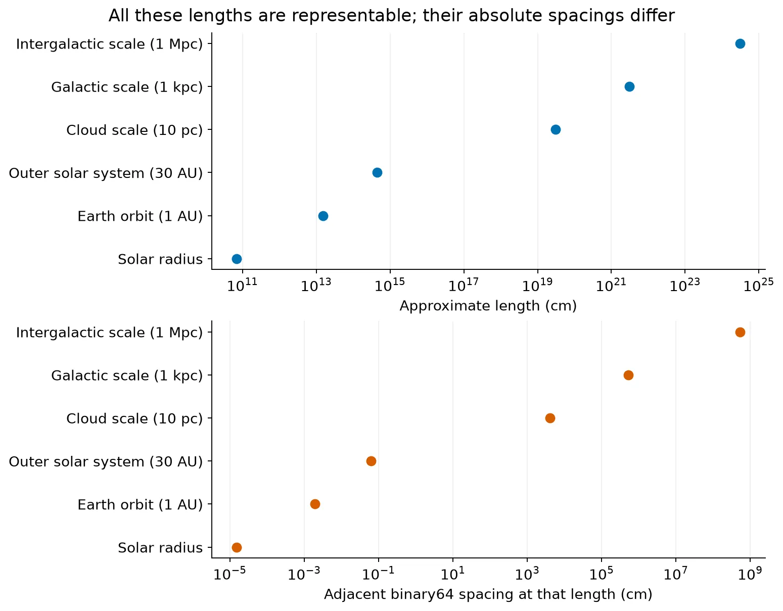
Figure 1:The upper panel shows approximate length scales, all readily representable in binary64. The lower panel shows the spacing to the next larger binary64 value at each scale. These are different quantities: representing a large position does not imply resolving a very small displacement added to it. The cloud, galactic, and intergalactic lengths are illustrative scales, not measurements of particular objects.
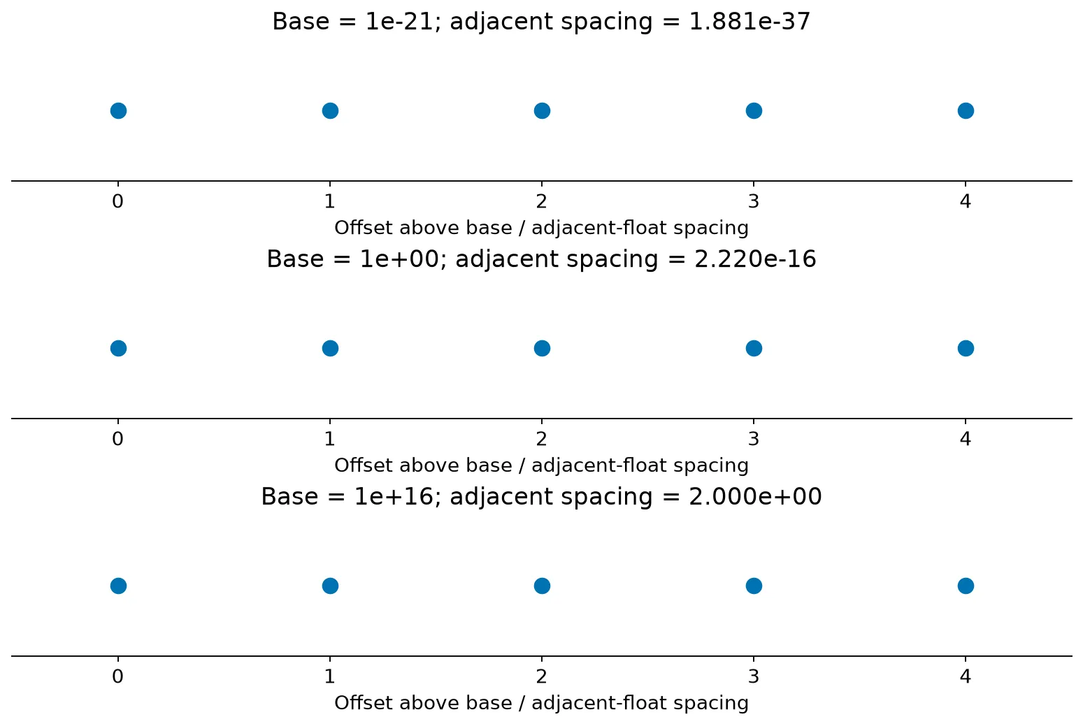
Figure 2:What to notice in this figure: representable numbers are discrete rather than continuous, and the gap between adjacent floating-point values grows with magnitude. That is why a subtraction that is safe near 1 may be ill-conditioned near 1016.
The takeaway is that scale is part of the numerical problem. The same subtraction can be harmless at one magnitude and poorly conditioned at another.
Finding Machine Epsilon
Why this matters: machine epsilon is the local scale at which a floating-point number near 1 stops changing when you perturb it.
NumPy defines machine epsilon as the distance from 1 to the next larger representable number:
Under round-to-nearest, a perturbation just larger than half this spacing can already change the rounded sum. Therefore, “the smallest positive number that changes 1 when added” is not the same definition. The halving experiment below searches powers of two and recovers the spacing, not every possible perturbation. NumPy’s definition.
For IEEE 754 double precision, the value is about
This means that near numbers of order unity, relative perturbations much smaller than 10-16 are typically invisible in double precision.
Worked Example 1: Why 0.1 + 0.2 != 0.3
Why this matters: this is the simplest way to see that floating-point numbers are binary approximations, not exact decimal objects.
What quantity is being computed?
A Boolean equality test and the stored floating-point representations of
0.1,0.2, and0.3.
What is known exactly?
The mathematical decimal numbers 0.1, 0.2, and 0.3 are exact real numbers in base 10 notation.
What is represented approximately on the computer?
Their nearest binary floating-point approximations in double precision.
What does the error mean in practice?
Exact equality checks on floating-point numbers can fail even when the printed decimals look simple and familiar.
def describe_float(value: float) -> tuple[int, int]:
    """Return the exact numerator and denominator of a Python float."""
    return value.as_integer_ratio()


values = [0.1, 0.2, 0.3, 0.1 + 0.2]
for value in values:
    numerator, denominator = describe_float(value)
    print(
        f"value = {value!r:<20} stored as {numerator}/{denominator} "
        f"= {numerator / denominator:.17f}"
    )

print(f"0.1 + 0.2 == 0.3 -> {(0.1 + 0.2) == 0.3}")
print(f"0.1 + 0.2        -> {0.1 + 0.2:.17f}")
print(f"0.3              -> {0.3:.17f}")
value = 0.1 stored as 3602879701896397/36028797018963968 = 0.10000000000000001
value = 0.2 stored as 3602879701896397/18014398509481984 = 0.20000000000000001
value = 0.3 stored as 5404319552844595/18014398509481984 = 0.29999999999999999
value = 0.30000000000000004 stored as 1351079888211149/4503599627370496 = 0.30000000000000004
0.1 + 0.2 == 0.3 -> False
0.1 + 0.2 -> 0.30000000000000004
0.3 -> 0.29999999999999999
Interpretation: the mismatch is not folklore and it is not a Python bug. The finite binary approximation of 0.1 is slightly different from the exact real number 0.1, and those tiny differences survive arithmetic.
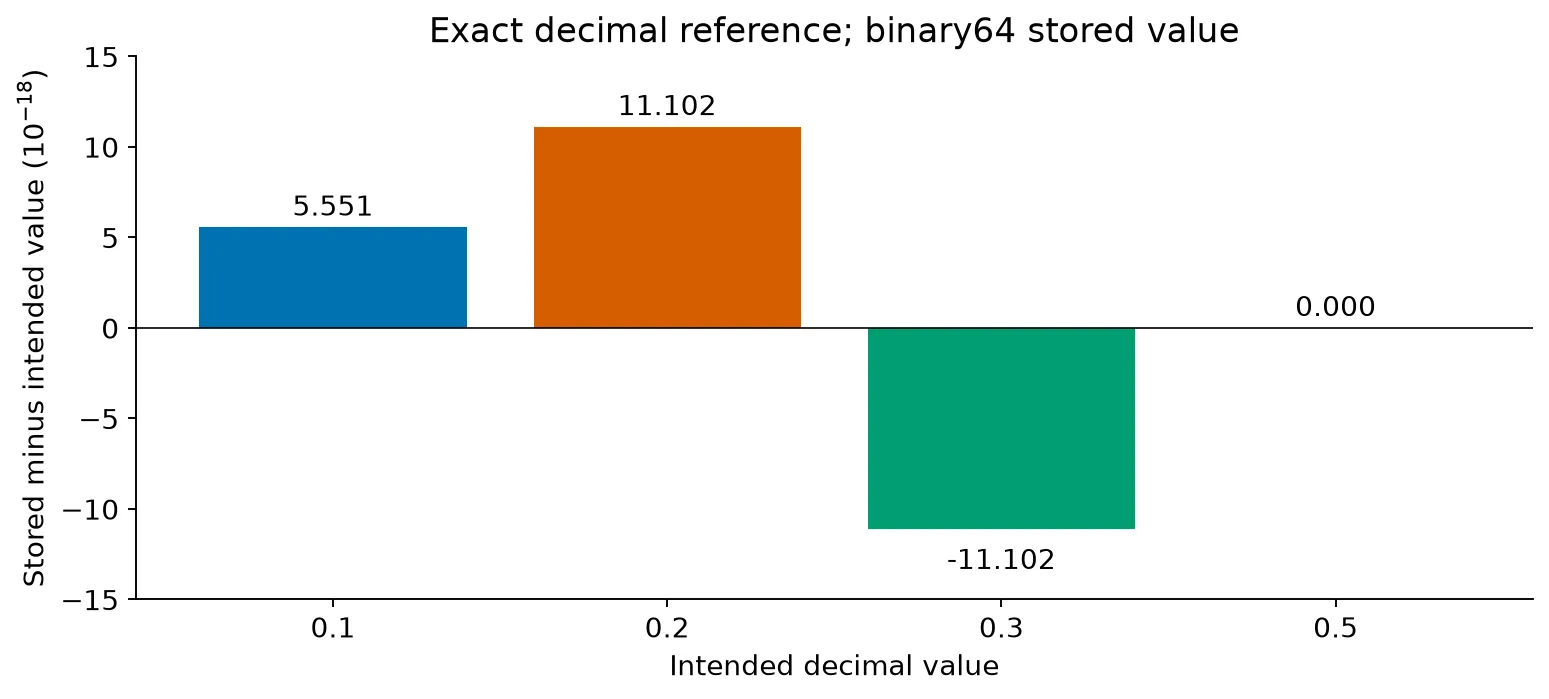
Figure 3:What to notice in this figure: the issue is not that the computer is careless. The issue is that most finite decimal fractions do not have finite binary expansions, so the stored values are the nearest available binary fractions.
Worked Example 2: Computing 
Why this matters: the abstract definition of machine epsilon becomes much easier to trust once you compute it yourself and compare it to NumPy’s built-in value.
What quantity is being computed?
for double precision.
What is known exactly?
NumPy reports the reference value through
np.finfo(float).eps.
What is represented approximately on the computer?
Each trial perturbation in the halving loop is itself a floating-point number.
What does the error mean in practice?
This tells you the spacing near 1. The useful refinement limit for a method depends on how its operations amplify rounding; it need not equal epsilon.
import math
from typing import Iterable

import numpy as np


def find_machine_epsilon() -> float:
    """Return the machine epsilon for Python float (double precision)."""
    eps = 1.0
    while (1.0 + eps / 2.0) != 1.0:
        eps /= 2.0
    return eps


eps_loop = find_machine_epsilon()
eps_numpy = np.finfo(float).eps
print(f"Loop result:   {eps_loop:.18e}")
print(f"NumPy result:  {eps_numpy:.18e}")
print(f"Relative gap:  {abs(eps_loop - eps_numpy) / eps_numpy:.3e}")
Loop result: 2.220446049250313081e-16
NumPy result: 2.220446049250313081e-16
Relative gap: 0.000e+00
Interpretation: the loop and the library agree because both are describing the same hardware-level double-precision format. The result is approximately , not exactly 10-16, because binary floating-point spacing is not organized in decimal powers.
Machine epsilon is a local spacing scale, not a universal error budget.
The Three Types of Error
Why this matters: students often treat all numerical error as one fuzzy category, but different errors come from different causes and require different fixes.
Representation Error: Round-off Error
Why this matters: if the computer cannot represent a number exactly, error is present before your algorithm even begins.
Student mental model: round-off error is a storage problem. The value you wanted and the value the computer stores are nearby, but not identical.
We can write the local scale of round-off influence schematically as
This equation says that representation error is tied to floating-point spacing, though the proportionality constant depends strongly on the problem and the operation being performed.
Algorithmic Approximation Error: Truncation Error
Why this matters: even with exact arithmetic, many scientific algorithms intentionally approximate an infinite process with a finite one.
Student mental model: truncation error is an algorithm-design problem. You stop a series, discretize a derivative, or take a finite timestep, and that choice introduces approximation error.
For a method of order , a standard local model is
This equation says that the error decreases as the resolution parameter shrinks, provided you are in the regime where the asymptotic model actually applies.
Accumulation and Amplification Error
Why this matters: a tiny per-step error can still become scientifically important if the computation repeats the step many times or amplifies perturbations dynamically.
Student mental model: propagation error is a history problem. The error you make now can be carried, accumulated, or magnified by everything that happens later.
If the signs of individual errors behave roughly like independent random kicks, a common model is
This equation says that random-sign accumulation behaves like a random walk, so the total error grows more slowly than linearly with the number of steps .
If the bias is coherent from step to step, a conservative model is
This equation says that systematic bias can accumulate linearly with the number of steps, which is much more dangerous for long integrations.
The takeaway is that different error sources call for different fixes. Better algebra, better resolution, and better diagnostics solve different problems.
Catastrophic Cancellation
Why this matters: catastrophic cancellation is the signature failure mode of subtracting nearly equal numbers in floating-point arithmetic.
Student mental model: when two nearly equal numbers are subtracted, the leading digits cancel and the remaining digits may contain very little reliable information. The problem is not the subtraction itself; the problem is that the subtraction exposes the least accurate part of both inputs.
Worked Example 3: A Stable and Unstable Parallax-Like Difference
Why this matters: astronomy often asks us to compare nearby distances, inverse distances, or optical-depth-like quantities where the naive algebra is numerically brittle.
What quantity is being computed?
The difference between two inverse distances, measured here in .
What is known exactly?
The two algebraic expressions are mathematically equivalent.
What is represented approximately on the computer?
The floating-point values of , , and their reciprocal evaluations.
What does the error mean in practice?
A naive formula can lose significant digits and make a small astrophysical signal look noisier or less trustworthy than it should.
def _validate_positive_finite_distance(name: str, value: float) -> float:
    """Validate a positive finite distance value."""
    scalar = float(value)
    if not np.isfinite(scalar) or scalar <= 0.0:
        raise ValueError(f"{name} must be a positive finite distance.")
    return scalar


def parallax_bad(d1: float, d2: float) -> float:
    """Return a naive difference of reciprocals."""
    d1_checked = _validate_positive_finite_distance("d1", d1)
    d2_checked = _validate_positive_finite_distance("d2", d2)
    return 1.0 / d1_checked - 1.0 / d2_checked


def parallax_good(d1: float, d2: float) -> float:
    """Return the algebraically equivalent but numerically safer form."""
    d1_checked = _validate_positive_finite_distance("d1", d1)
    d2_checked = _validate_positive_finite_distance("d2", d2)
    return (d2_checked - d1_checked) / (d1_checked * d2_checked)
d1_au = 1.000000000000000
d2_au = 1.000000000000067
bad_value = parallax_bad(d1_au, d2_au)
good_value = parallax_good(d1_au, d2_au)
relative_difference = abs(bad_value - good_value) / abs(good_value)
print(f"Naive value: {bad_value:.18e} AU^-1")
print(f"Stable value: {good_value:.18e} AU^-1")
print(f"Relative gap: {relative_difference:.3e}")Naive value: 6.705747068735945504e-14 AU^-1
Stable value: 6.705747068735496169e-14 AU^-1
Relative gap: 6.701e-14
Interpretation: the reformulation subtracts the stored distances directly, before rounding two reciprocal evaluations. Nearby floating-point distances can subtract exactly even though they approximate the intended decimal inputs. To see what the algebra repairs, we need two references: the intended decimal problem and the problem defined by the stored binary inputs.
from decimal import Decimal, localcontext

with localcontext() as context:
    context.prec = 70
    # Decimal strings describe the intended data; from_float preserves stored bits.
    d1_decimal = Decimal("1.000000000000000")
    d2_decimal = Decimal("1.000000000000067")
    decimal_reference = 1 / d1_decimal - 1 / d2_decimal
    d1_binary = Decimal.from_float(d1_au)
    d2_binary = Decimal.from_float(d2_au)
    binary_reference = 1 / d1_binary - 1 / d2_binary
    input_error = abs(binary_reference - decimal_reference)
    bad_error = abs(Decimal.from_float(bad_value) - binary_reference)
    good_error = abs(Decimal.from_float(good_value) - binary_reference)
    print(f"Input representation contribution: {input_error:.3E} AU^-1")
    print(f"Naive evaluation error:            {bad_error:.3E} AU^-1")
    print(f"Reformulated evaluation error:     {good_error:.3E} AU^-1")
    for name, value in (("naive", bad_value), ("reformulated", good_value)):
        total_error = abs(Decimal.from_float(value) - decimal_reference)
        print(f"Total error against decimal data ({name}): {total_error:.3E}")
Input representation contribution: 5.747E-17 AU^-1
Naive evaluation error: 4.497E-27 AU^-1
Reformulated evaluation error: 3.353E-30 AU^-1
Total error against decimal data (naive): 5.747E-17
Total error against decimal data (reformulated): 5.747E-17
The reformulated expression evaluates the stored-input problem more accurately. The total errors against the intended decimals remain nearly equal because the input representation contribution dominates. Algebra cannot recover information already lost when the distances were stored. This distinction matters when a code improvement appears to have no effect on the final scientific observable.
Check Your Understanding — answer
Would increasing only the arithmetic precision after reading the distances as ordinary floats restore the intended decimals? No. It preserves those already rounded inputs more accurately. To reduce input representation error as well, the higher-precision calculation must begin with the original decimal strings.
Stable Reformulation
Why this matters: when a numerical expression is fragile, the first fix is often algebraic rather than algorithmic.
Another classic example is
This equation says that if and are close, the left-hand side performs two unstable operations before dividing, while the right-hand side avoids the cancellation entirely.
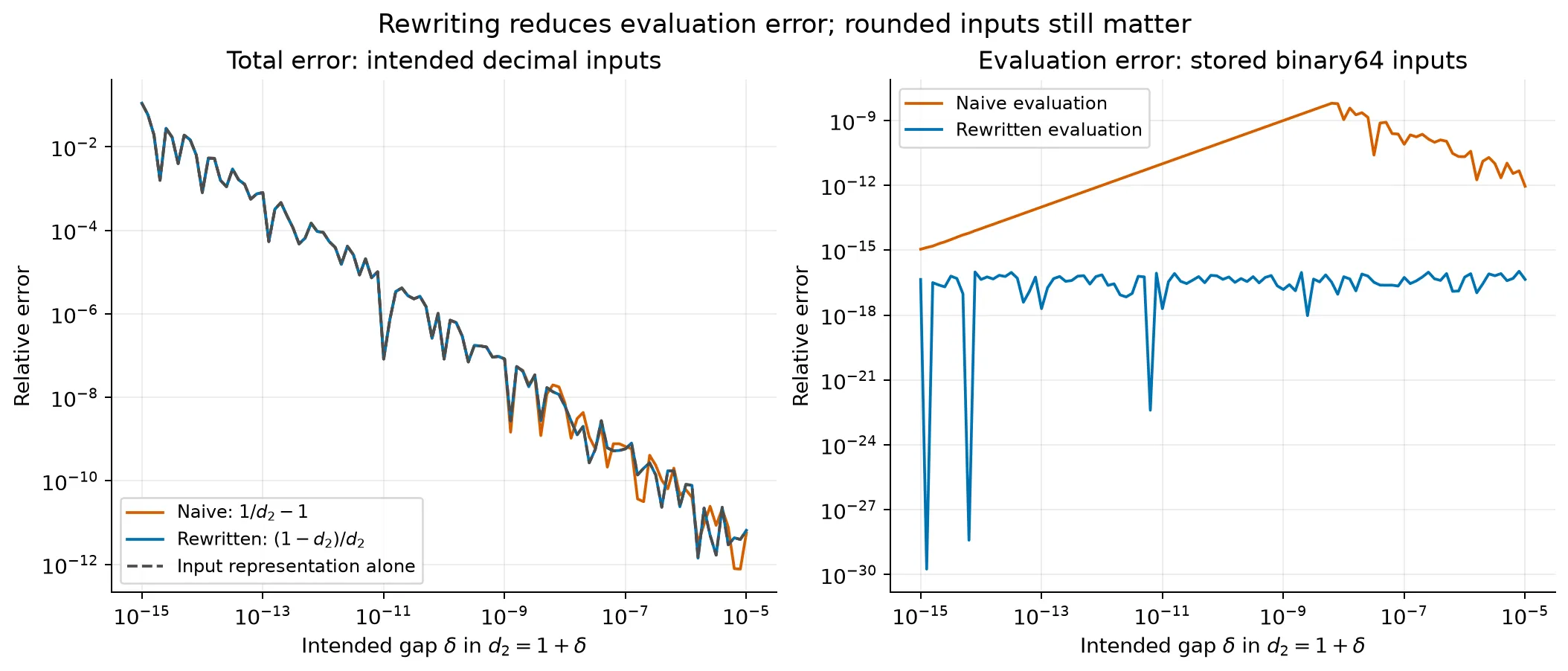
Figure 4:The intended dimensionless inputs are and . Both formulas use the same stored binary64 inputs. The left panel compares their answers with a 90-digit decimal reference for the intended inputs; the right uses a 90-digit reference for the stored inputs. Rewriting the reciprocal difference reduces evaluation error to about floating-point precision, but it cannot recover the input digits already lost when storing . Consequently, the total errors can remain comparable. No artificial error floor is plotted.
Algebraic equivalence does not imply numerical equivalence. Catastrophic cancellation is a conditioning problem exposed by subtraction.
Measuring Errors: Absolute vs. Relative
Why this matters: the same numerical difference can be negligible in one context and catastrophic in another.
We define absolute error by
This equation measures the raw size of the discrepancy in the physical units of the quantity itself.
We define relative error by
This equation measures the discrepancy relative to the size of the true value, which is often more meaningful away from zero.
def absolute_relative_error(
    computed: float,
    true: float,
    zero_scale: float | None = None,
) -> dict[str, float | str]:
    """Return absolute and relative error with a near-zero decision rule."""
    computed_scalar = float(computed)
    true_scalar = float(true)

    if not np.isfinite(computed_scalar) or not np.isfinite(true_scalar):
        raise ValueError("computed and true must both be finite.")

    if zero_scale is not None:
        zero_scale_scalar = float(zero_scale)
        if not np.isfinite(zero_scale_scalar) or zero_scale_scalar <= 0.0:
            raise ValueError("zero_scale must be a positive finite value when provided.")
    else:
        zero_scale_scalar = 1.0

    absolute_error = abs(computed_scalar - true_scalar)
    near_zero_threshold = np.sqrt(np.finfo(float).eps) * zero_scale_scalar

    # Relative error is mathematically undefined only at an exactly zero reference.
    relative_error = math.nan if true_scalar == 0.0 else absolute_error / abs(true_scalar)
    recommended_metric = "absolute" if abs(true_scalar) <= near_zero_threshold else "relative"

    return {
        "absolute_error": absolute_error,
        "relative_error": relative_error,
        "recommended_metric": recommended_metric,
        "near_zero_threshold": near_zero_threshold,
    }
The threshold in this helper is an illustrative reporting heuristic, not a definition of zero or an acceptance tolerance. It does not suppress a defined relative error: for a nonzero reference of 10-8 and a computed value of , the relative error is 1, or 100%. Whether that matters requires a physical accuracy target.
Worked Example 4: Computing Jupiter’s Mass
Why this matters: a large absolute difference can still be an excellent result if the reference quantity is enormous.
What quantity is being computed?
The error in a computed value of Jupiter’s mass.
What is known exactly?
For this worked example, we take the reference value
as the accepted true value.
What is represented approximately on the computer?
The computed value
What does the error mean in practice?
It shows how absolute and relative error can tell very different stories about the same numerical result.
The absolute error is
This equation says the raw discrepancy is one thousand trillion trillion grams, which sounds enormous until we compare it with Jupiter’s full mass.
The relative error is
This equation says the computation is wrong by only about five-hundredths of a percent, which is excellent for many astrophysical purposes.
jupiter_true_g = 1.898e30
jupiter_computed_g = 1.897e30
jupiter_errors = absolute_relative_error(jupiter_computed_g, jupiter_true_g)

print(f"Absolute error: {jupiter_errors['absolute_error']:.3e} g")
print(f"Relative error: {jupiter_errors['relative_error']:.3e}")
print(f"Recommended metric: {jupiter_errors['recommended_metric']}")
Absolute error: 1.000e+27 g
Relative error: 5.269e-04
Recommended metric: relative
Interpretation: the absolute error is physically large because Jupiter is physically large. The relative error is the better summary here because the true value is nowhere near zero.
Worked Example 5: Near-Zero Failure of Relative Error
Why this matters: near zero, relative error can look dramatic even when the physical discrepancy is negligible.
What quantity is being computed?
The error in a nearly zero center-of-mass radial velocity.
What is known exactly?
For this worked example, we take
as the reference value.
What is represented approximately on the computer?
The computed value
What does the error mean in practice?
The relative error is , but the physical mismatch is only , which may be negligible in a large simulation.
v_true = 1.0e-8  # cm s^-1
v_computed = 2.0e-8  # cm s^-1
velocity_errors = absolute_relative_error(v_computed, v_true, zero_scale=1.0e5)

print(f"Absolute error:      {velocity_errors['absolute_error']:.3e} cm s^-1")
print(f"Relative error:      {velocity_errors['relative_error']:.3e}")
print(f"Recommended metric:  {velocity_errors['recommended_metric']}")
Absolute error: 1.000e-08 cm s^-1
Relative error: 1.000e+00
Recommended metric: absolute
Interpretation: the relative error sounds catastrophic because the denominator is tiny. In practice, the absolute error may be the more meaningful diagnostic when the physically relevant baseline is close to zero.
import matplotlib.pyplot as plt


regime_names = ["Jupiter mass (g)", "dimensionless quantity", "velocity (cm/s)"]
true_values = np.array([1.898e30, 1.0, 1.0e-8])
computed_values = np.array([1.897e30, 0.95, 2.0e-8])
absolute_errors = np.abs(computed_values - true_values)
relative_errors = absolute_errors / np.abs(true_values)

fig, axes = plt.subplots(2, 1, figsize=(8.5, 5.8), sharex=True)
x_positions = np.arange(len(regime_names))
palette = [plt.get_cmap("tab10")(idx) for idx in range(len(regime_names))]

axes[0].scatter(x_positions, absolute_errors, s=55, color=palette)
axes[0].set_yscale("log")
axes[0].set_ylabel("Numeric absolute error\n(in each example's units)")
axes[0].set_title("Separate examples: absolute errors have different units")

axes[1].scatter(x_positions, relative_errors, marker="s", s=55, color=palette)
axes[1].set_yscale("log")
axes[1].set_ylabel(r"$E_{\mathrm{rel}}$")
axes[1].set_title("Relative error across the same three regimes")
axes[1].set_xticks(x_positions, regime_names, rotation=15)

for ax in axes:
    ax.grid(True, axis="y", alpha=0.25)

fig.tight_layout()
plt.show()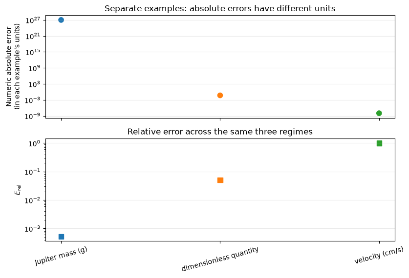
What to notice: the top panel shows three separate numerical examples in their stated units. A mass error in grams cannot be ranked physically against a velocity error in centimeters per second by comparing these numbers. The bottom panel uses dimensionless relative errors, which allow a fractional comparison across scales. The near-zero reference still needs care: a large fractional error can correspond to a small absolute discrepancy. Whether that discrepancy matters depends on the physical accuracy required.
Relative error is powerful away from zero and often misleading near zero.
From measured errors to atol and rtol
An error measures a discrepancy. A tolerance states how much discrepancy a particular comparison permits. Increasing the tolerance changes the decision, not the computed result. We should choose it from a physical target, a method error bound, or a justified numerical comparison before seeing whether a test passes.
For finite values, NumPy’s isclose(computed, reference, rtol=r, atol=a) tests
The reference belongs second: NumPy uses it for the relative scale. atol has
the quantity’s units, while rtol is dimensionless (0.01 means 1%). The
allowances add; passing does not mean satisfying both limits separately.
At zero reference only atol contributes. NumPy comparison semantics.
Predict: the following residuals are in centimeters. The example’s stated
criterion allows 10-8 cm plus one part in a million of the reference.
Which rows pass? Write the allowed error before calling np.isclose.
reference_cm = np.array([0.0, 1.0, 1.0e6])
computed_cm = reference_cm + np.array([3.0e-9, 0.1, 0.1])
atol_cm, rtol = 1.0e-8, 1.0e-6  # Stated targets for this example, not defaults.
errors_cm = np.abs(computed_cm - reference_cm)  # Elementwise absolute values.
allowed_cm = atol_cm + rtol * np.abs(reference_cm)
print("absolute errors [cm]:", errors_cm)
print("allowed errors [cm]: ", allowed_cm)
print("accepted:", np.isclose(computed_cm, reference_cm, rtol=rtol, atol=atol_cm))
print("zero, relative only:", np.isclose(3e-9, 0.0, rtol=rtol, atol=0.0))
print("tiny reference, defaults:", np.isclose(2e-12, 1e-12))
print("tiny reference, 1%:", np.isclose(2e-12, 1e-12, rtol=0.01, atol=0.0))
absolute errors [cm]: [3.e-09 1.e-01 1.e-01]
allowed errors [cm]: [1.00000000e-08 1.01000000e-06 1.00000001e+00]
accepted: [ True False True]
zero, relative only: False
tiny reference, defaults: True
tiny reference, 1%: False
The first and third rows pass, for different reasons. At zero, the absolute allowance accepts the residual; at 106 cm the relative allowance is about 1 cm. The same 0.1 cm discrepancy fails at 1 cm. The tiny-reference example shows why defaults deserve scrutiny: a 100% relative error passes when the default absolute allowance is much larger than either value.
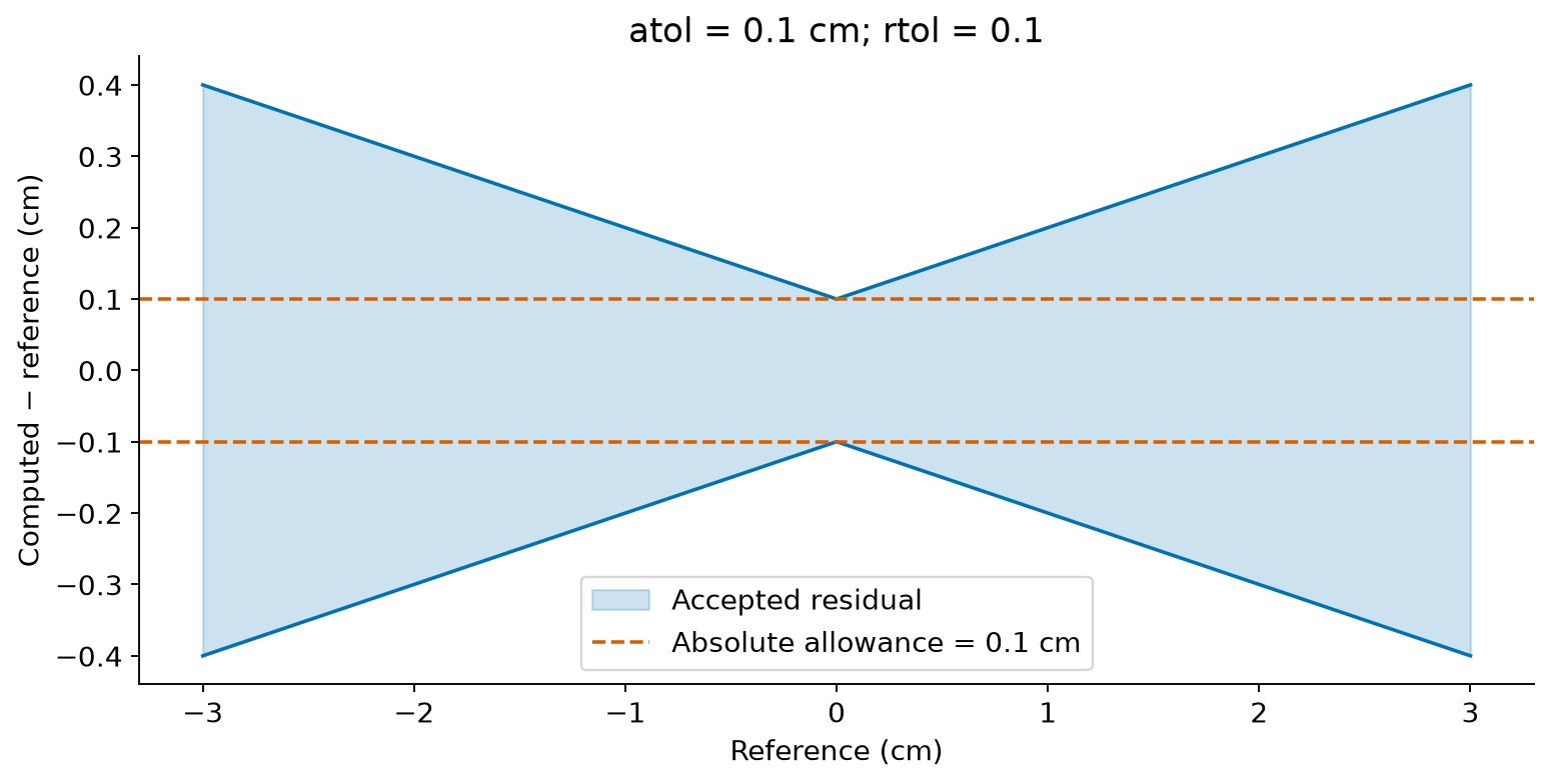
The boundary is .
The plotted example uses atol=0.1 cm and rtol=0.1 so both contributions are
visible. They are illustrative scales, not recommended course-wide tolerances.
np.isclose works element by element; np.allclose requires all comparisons
to pass. Check array shapes so broadcasting does not silently compare the wrong
objects. Also check finiteness when your mathematical model requires finite
values: a closeness test is not a complete input or result validation.
Lecture 1’s math.isclose uses a different rule for finite scalars:
. It is symmetric and
takes a maximum rather than a sum. Read the API rather than assuming a rename
preserves the criterion. In pytest.approx, the allowance is also a maximum
of its supplied absolute and expected-value-scaled relative tolerances.
Check Your Understanding — tolerance or method?
If a first-order quadrature rule misses the target, setting rtol=1e-12 does
not improve it. Increase resolution, choose a more suitable rule, or repair
the integrand evaluation, then measure again. If the reference is itself
approximate, the discrepancy includes its error; budget for that uncertainty
rather than treating a library result as exact.
Tracking Accumulated Error
Why this matters: long-running simulations care not just about per-step error, but about what happens to those errors after thousands, millions, or billions of updates.
Worked Example 6: Error Propagation Over Many Steps
Why this matters: repeated updates can turn an individually tiny error into a meaningful drift.
What quantity is being computed?
Model accumulated error after repeated updates.
What is known exactly?
We prescribe the per-step error model rather than measuring a hidden true trajectory.
What is represented approximately on the computer?
The cumulative effect of small errors over many steps.
What does the error mean in practice?
It tells you why long integrations require stronger diagnostics than one-step calculations.
def demonstrate_error_propagation(
    step_counts: Iterable[int],
    per_step_error: float = np.finfo(float).eps,
) -> list[dict[str, float]]:
    """Return random and systematic accumulation models for a set of step counts."""
    per_step_error_scalar = float(per_step_error)
    if not np.isfinite(per_step_error_scalar) or per_step_error_scalar <= 0.0:
        raise ValueError("per_step_error must be a positive finite number.")

    results: list[dict[str, float]] = []
    for step_count in step_counts:
        step_count_int = int(step_count)
        if step_count_int <= 0:
            raise ValueError("All step counts must be positive integers.")

        random_walk_model = np.sqrt(step_count_int) * per_step_error_scalar
        systematic_model = step_count_int * per_step_error_scalar
        results.append(
            {
                "step_count": float(step_count_int),
                "random_walk_error": random_walk_model,
                "systematic_error": systematic_model,
            }
        )
    return results
propagation_results = demonstrate_error_propagation([1, 10, 100, 10_000, 1_000_000])
for row in propagation_results:
print(
f"steps = {int(row['step_count']):>8d} "
f"random model = {row['random_walk_error']:.3e} "
f"systematic model = {row['systematic_error']:.3e}"
)steps = 1 random model = 2.220e-16 systematic model = 2.220e-16
steps = 10 random model = 7.022e-16 systematic model = 2.220e-15
steps = 100 random model = 2.220e-15 systematic model = 2.220e-14
steps = 10000 random model = 2.220e-14 systematic model = 2.220e-12
steps = 1000000 random model = 2.220e-13 systematic model = 2.220e-10
Interpretation: the random-walk model grows more slowly because positive and negative errors partially cancel. The systematic model grows faster because every step pushes in the same direction.
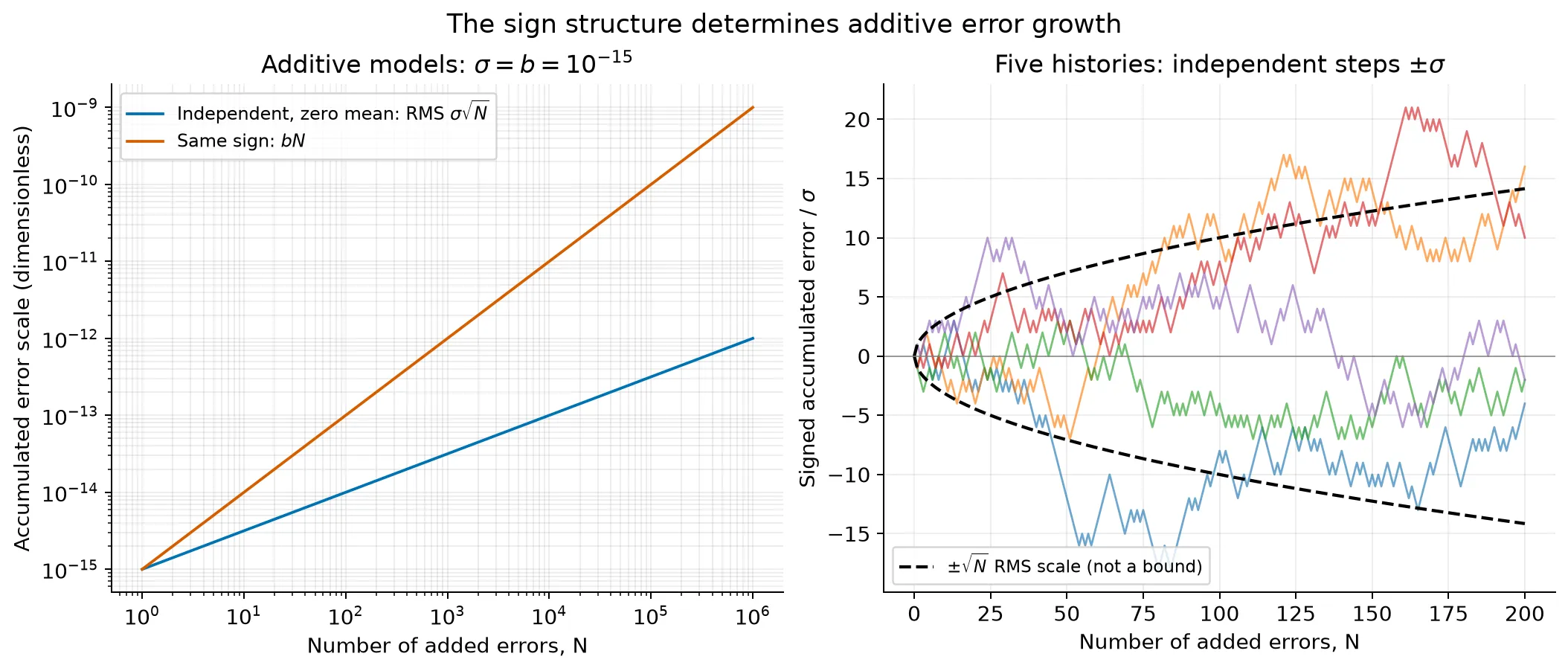
Figure 6:These are additive models with the illustrative dimensionless scale : independent zero-mean errors with standard deviation give RMS accumulated error , while identical positive errors give . The five seeded histories use independent steps ; the dashed RMS scale is not a bound on a history. The models contain no dynamical amplification and do not prescribe tolerances from simulation duration.
The takeaway is that repeated tiny errors matter because history matters. Growth law, sign structure, and amplification all change the scientific risk.
Adaptive Error Control
Why this matters: many algorithms cannot afford to run with a single fixed step size or tolerance everywhere.
Suppose an error estimator gives a current value . A basic tolerance rule is
This equation says that if the estimated error exceeds the target tolerance, the current resolution is not adequate.
For a method of order , a typical controller uses
This equation says that higher estimated error should trigger a smaller next step, with the exact exponent depending on the error model of the method.
The simplified helper below is only a heuristic controller, not a universal adaptive-step law.
In a real solver, the controller exponent and update logic depend on the method and the error estimator, so this helper is illustrative rather than canonical.
def adaptive_h(error_estimate: float, h_current: float, tolerance: float) -> float:
    """Adjust step size based on a simple second-order-style safety controller."""
    error_estimate_scalar = float(error_estimate)
    h_current_scalar = float(h_current)
    tolerance_scalar = float(tolerance)

    if not np.isfinite(error_estimate_scalar) or error_estimate_scalar < 0.0:
        raise ValueError("error_estimate must be a finite non-negative value.")
    if not np.isfinite(h_current_scalar) or h_current_scalar <= 0.0:
        raise ValueError("h_current must be a positive finite value.")
    if not np.isfinite(tolerance_scalar) or tolerance_scalar <= 0.0:
        raise ValueError("tolerance must be a positive finite value.")

    if error_estimate_scalar == 0.0:
        return 2.0 * h_current_scalar

    if error_estimate_scalar > tolerance_scalar:
        shrink_factor = max(0.1, 0.9 * np.sqrt(tolerance_scalar / error_estimate_scalar))
        return h_current_scalar * shrink_factor

    if error_estimate_scalar < tolerance_scalar / 4.0:
        grow_factor = min(2.0, 0.9 * np.sqrt(tolerance_scalar / error_estimate_scalar))
        return h_current_scalar * grow_factor

    return h_current_scalar
h_current = 0.1
for estimated_error in [1.0e-2, 5.0e-5, 0.0]:
h_new = adaptive_h(estimated_error, h_current=h_current, tolerance=1.0e-4)
print(f"estimated error = {estimated_error:.1e} h_new = {h_new:.3e}")estimated error = 1.0e-02 h_new = 1.000e-02
estimated error = 5.0e-05 h_new = 1.000e-01
estimated error = 0.0e+00 h_new = 2.000e-01
Interpretation: a large error estimate reduces the step size, a very small one allows a larger step, and the zero-error case is treated cautiously rather than dividing by zero.
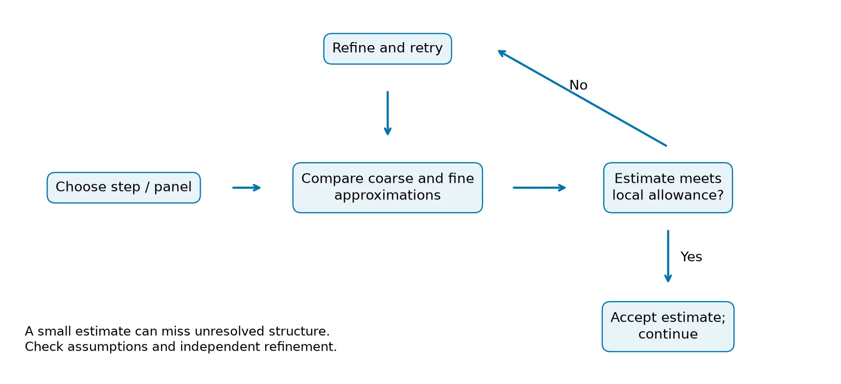
Figure 7:Adaptive control is a feedback loop. The algorithm changes its step size in response to an error estimate, trading computational work against a stated accuracy target.
The takeaway is that adaptive control is a method-specific feedback design, not a single rule to memorize.
Error Tolerances in Practice
Why this matters: students often want a single “correct tolerance,” but useful targets depend on the quantity being monitored, the scale of the physics, and the scientific question.
The table below gives context-dependent examples, not universal commandments. It is also not a set of values to memorize. It is meant to help you ask better questions about scale, diagnostics, and scientific purpose.
| Application | Typical Numerical Target | Why That Target Is Chosen | Cautionary Note |
|---|---|---|---|
| Quadrature benchmark | A tolerance justified by the rule’s observed order and the exact reference | The sine integral and make a measured error possible | A test tolerance must be looser than the expected numerical error but tight enough to catch a broken rule |
| Long conservative integration | Problem-dependent conservation monitor plus convergence study | Long runs accumulate error, so invariants and cross-resolution checks matter together | A single scalar tolerance is rarely enough |
| Stellar structure or evolution solve | Residuals around 10-6 to 10-8, depending on model and solver | Often below dominant input-physics uncertainty while still numerically stable | Do not confuse solver tolerance with physical uncertainty |
| Galaxy or cluster simulation | Global conservation and ensemble statistics at about 10-4 to 10-6, depending on the observable | Often the global structure matters more than trajectory-level perfection | Particle-level exactness is usually not the goal |
| MCMC sampling | Diagnostics such as and adequate effective sample size | Sampling quality is assessed statistically rather than by one floating-point tolerance | Detailed balance is a property of the algorithm, not a “tolerance row” |
| Gradient-based optimization | Relative loss or gradient norm threshold around 10-6 or a problem-scaled stopping rule | Useful when further iterations do not change the model meaningfully | Stop criteria should reflect model scale and noise, not just machine precision |
Interpretation: numerical targets are chosen to answer a scientific question reliably, not to win a contest for the smallest printed number.
Convergence Testing Without True Values
Why this matters: in research code, you often do not know the true answer. You need a way to test whether refinement is behaving consistently with the order of the method.
This section combines three related but different ideas:
exact-reference testing, when you know the answer and can compare directly,
self-convergence testing, when you compare multiple resolutions to each other,
Richardson-style error estimation, when you convert those resolution differences into an estimated finer-grid error.
Suppose the leading error behaves like
where is the order of the method.
This equation says that halving should reduce the leading error by about a factor of once the solution is in the asymptotic regime.
If you compute the same quantity at two resolutions, and , then a Richardson-style estimate is
This equation says that the difference between two resolutions can estimate the error of the finer one when the asymptotic model is valid.
def central_difference_sine(x: float, h: float) -> float:
    """Return the central-difference derivative of sin(x) at one point."""
    if not np.isfinite(x):
        raise ValueError("x must be finite.")
    if not np.isfinite(h) or h <= 0.0:
        raise ValueError("h must be a positive finite value.")
    return (np.sin(x + h) - np.sin(x - h)) / (2.0 * h)


x_eval = 1.0
p = 2
h_values = [1.0e-1, 5.0e-2, 2.5e-2, 1.25e-2]
approximations = [central_difference_sine(x_eval, h) for h in h_values]
differences = [
    abs(approximations[i] - approximations[i + 1])
    for i in range(len(approximations) - 1)
]

for h_value, approximation in zip(h_values, approximations):
    print(f"h = {h_value:.5f}  approximation = {approximation:.12f}")

print("\nSuccessive-difference ratios:")
for i in range(len(differences) - 1):
    ratio = differences[i] / differences[i + 1]
    print(
        f"ratio between h = {h_values[i]:.5f} and h = {h_values[i+1]:.5f}: {ratio:.3f}"
    )

print("\nRichardson-style error estimates for the finer solution:")
for i in range(len(approximations) - 1):
    estimated_error = differences[i] / (2**p - 1)
    print(
        f"fine h = {h_values[i+1]:.5f}  "
        f"E_estimated = {estimated_error:.3e}"
    )
h = 0.10000 approximation = 0.539402252170
h = 0.05000 approximation = 0.540077208046
h = 0.02500 approximation = 0.540246026137
h = 0.01250 approximation = 0.540288235606
Successive-difference ratios:
ratio between h = 0.10000 and h = 0.05000: 3.998
ratio between h = 0.05000 and h = 0.02500: 4.000
Richardson-style error estimates for the finer solution:
fine h = 0.05000 E_estimated = 2.250e-04
fine h = 0.02500 E_estimated = 5.627e-05
fine h = 0.01250 E_estimated = 1.407e-05
Interpretation: for a second-order method, the successive-difference ratios should trend toward in the asymptotic regime. If they do not, you should check whether round-off, non-smoothness, or implementation bugs are interfering.
Convergence tests check whether the method behaves like the theory predicts, not whether one number merely looks plausible.
Bridge to Part 3
Why this matters: this lesson handled the arithmetic side of numerical error, but not yet the full approximation model of a discretized method.
Part 2 gave us a language for representation error, cancellation, error metrics, accumulation, and tolerance logic. Part 3 adds the Taylor-series viewpoint that models truncation error directly and shows why different finite-difference formulas have different orders.
The key connection is this:
Part 2 explains how floating-point representation and repeated computation distort results.
Part 3 explains how Taylor expansions predict the truncation structure of numerical methods.
Part 3 unifies these ideas by showing how a real computation lives at the intersection of approximation error and floating-point error.
The takeaway to carry forward is that numerical trust comes from both arithmetic awareness and approximation theory.
Next: Part 3 - Taylor Series