Part 1: The Failure of Naive Integration - COMP 521: Introduction to Scientific Computing and Data Science

Learning Objectives¶

By the end of this section, you will be able to:

Implement Euler’s method and witness its catastrophic energy drift
Analyze local vs global error accumulation through Taylor series
Understand why higher accuracy doesn’t guarantee better long-term behavior
Recognize the geometric failure modes in phase space
Predict when and how integration methods will fail

From Continuous to Discrete¶

The fundamental ODE initial value problem asks us to find a function $x(t)$ given its rate of change:

\frac{dx}{dt} = f(x, t), \quad x(t_0) = x_0

(1)

This has the formal integral solution:

x(t) = x_0 + \int_{t_0}^t f(x(s), s) ds

(2)

Initial Value Problem (IVP): Finding a function given its derivative and starting value — the fundamental problem of dynamics.

But this Initial Value Problem contains a circular dependency: to find $x(t)$ , we need to integrate $f(x(s), s)$ , but $f$ depends on the unknown solution $x(s)$ itself!

Numerical methods break this circular dependency by making assumptions about how $f$ behaves over small time intervals:

Constant derivative assumption (Euler): Assume $f$ stays constant over $[t_n, t_{n+1}]$
Linear variation assumption (Trapezoidal): Assume $f$ varies linearly between endpoints
Matched intermediate stages (Runge-Kutta): Evaluate $f$ at predicted states so the update matches the solution Taylor expansion to a chosen order

Each assumption leads to a different family of methods with different error behaviors, stability properties, and conservation characteristics.

The Dimensional Analysis of Timesteps¶

Before diving into specific methods, let’s understand what constrains our choice of timestep $h$ from pure dimensional analysis.

For an oscillatory system, the dimensionless quantity $\omega h$ compares the step with the dynamical timescale. If $T=2\pi/\omega$ , then $h=0.1T$ gives 10 steps per period and $h=0.01T$ gives 100. Neither choice is an accuracy guarantee.

Sampling a prescribed band-limited signal above its Nyquist rate is a different problem from integrating its dynamics. An ODE method must also be stable: forward Euler is unstable on a pure oscillator for every nonzero $h$ , while leapfrog’s oscillator stability interval is $0<\omega h<2$ .

For gravitational systems, compare the orbital timescale $T=2\pi\sqrt{a^3/(GM)}$ with encounter scales such as $R/v_{\rm rel}$ and $\sqrt{R^3/[G(m_1+m_2)]}$ . Close encounters can introduce a much shorter scale than the main orbit. No fixed fraction of one timescale guarantees accuracy for every orbit, method, or requested observable.

Example — a one-year period: a one-day step gives about 365 steps per period; a tenth-day step gives about 3650. Both are candidate resolutions to compare, not labels meaning “ordinary” and “high” accuracy. Measure trajectory, energy, and phase errors under refinement over the actual duration you need.

Euler’s Method - The Simplest Approach¶

Mathematical Formulation¶

Euler’s method: The simplest ODE integration scheme, using a constant derivative over each timestep.

Euler’s method is the most straightforward discretization possible. Given the ODE

\frac{dx}{dt} = f(x,t),

(3)

at time $t_n$ with solution $x_n$ , and a timestep $h$ , we approximate:

\boxed{x_{n+1} = x_n + h f(x_n, t_n)}

(4)

This assumes the derivative $f$ remains constant over the entire interval $[t_n, t_{n+1}]$ — essentially extending the tangent line at $t_n$ forward by distance $h$ .

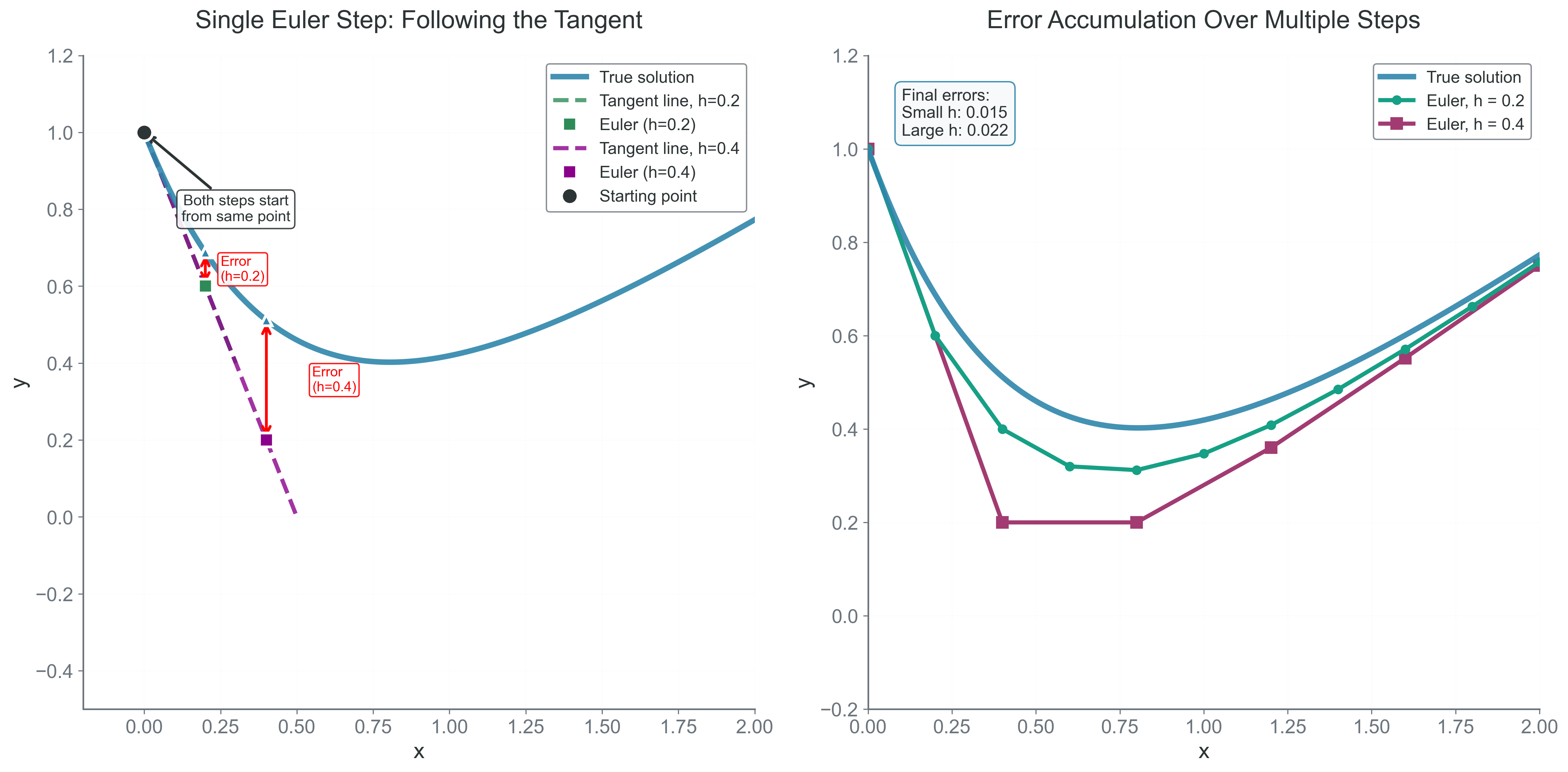
Euler's method extends the tangent line at each point, accumulating error by ignoring the solution's curvature — Figure 1:Euler’s method extends the tangent line at each point. This dimensionless example solves $y'=-2y+t$ , $y(0)=1$ , with exact reference $y(t)=\tfrac54e^{-2t}+\tfrac12t-\tfrac14$ (the figure labels the independent variable $x$ ). The left panel compares single steps; the right compares repeated steps through $t=2$ . The final absolute errors are about 0.01534 for $h=0.2$ and 0.02249 for $h=0.4$ . Error is not monotone in time here: it grows initially and then decreases. For a smooth problem over a fixed interval, Euler’s one-step error is $O(h^2)$ and its global error is $O(h)$ .

Taylor Series Analysis of Error¶

Local truncation error: Error introduced in a single step, assuming perfect starting values.

Global error: Total accumulated error over the entire integration interval.

To understand Euler’s error precisely, we need the Taylor series. The true solution at $t_{n+1} = t_n + h$ is:

x(t_n + h) = x(t_n) + h x'(t_n) + \frac{h^2}{2}x''(t_n) + \frac{h^3}{6}x'''(t_n) + O(h^4)

(5)

Since $x'(t_n) = f(x(t_n), t_n)$ by definition of our ODE, Euler’s method gives:

\boxed{x_{n+1} = x_n + h f(x_n, t_n)}

(6)

The local truncation error — the error in one step — is:

\tau_n = x(t_{n+1}) - x_{n+1} = \frac{h^2}{2}x''(t_n) + O(h^3)

(7)

The one-step defect is $O(h^2)$ ; Euler is called a first-order method because its global error is $O(h)$ on a fixed time interval under smoothness and stability assumptions. Global error is not generally the unweighted sum of the local defects: a wrong state changes the next derivative.

If $f$ is Lipschitz in the state with constant $L$ and each defect is bounded by $Ch^2$ , then, starting from an exact initial value,

|e_{n+1}|\le(1+hL)|e_n|+Ch^2,

(8)

and summing this geometric bound gives, for $L>0$ ,

|e_N|\le\frac{Ch}{L}\big[(1+hL)^N-1\big] \le\frac{Ch}{L}(e^{LT}-1),\qquad T=Nh.

(9)

For $L=0$ , the bound is $CTh$ . This explains the $O(h)$ global order at fixed $T$ and why the duration matters. Halving $h$ approximately halves the leading error only while that term dominates.

The Energy Drift Catastrophe¶

Let’s see Euler fail catastrophically on the harmonic oscillator:

\ddot{x} = -\omega^2 x

(10)

Converting to first-order system:

\frac{d}{dt}\begin{pmatrix} x \\ v \end{pmatrix} = \begin{pmatrix} v \\ -\omega^2 x \end{pmatrix}

(11)

The true solution has constant energy $E = \frac{1}{2}(v^2 + \omega^2 x^2).$

Implementation and Analysis¶

import numpy as np

def euler_harmonic(x0, v0, omega, h, n_steps):
    """Integrate harmonic oscillator with Euler's method"""
    x, v = x0, v0
    E0 = 0.5 * (v0**2 + omega**2 * x0**2)
    
    energies = [E0]
    for i in range(n_steps):
        # Euler update
        a = -omega**2 * x
        x = x + h * v
        v = v + h * a
        
        # Energy (should be constant, but...)
        E = 0.5 * (v**2 + omega**2 * x**2)
        energies.append(E)
    
    return energies

The energy increases at every step. For this oscillator we can derive the complete growth law, so there is no need to attach an unexplained percentage to a particular number of periods. The apparent linear growth at short times is the beginning of an exponential.

Mathematical Analysis of Energy Growth¶

For the harmonic oscillator with Euler’s method, we can derive the exact energy growth rate. Starting with position $x_n$ and velocity $v_n$ :

x_{n+1} = x_n + hv_n

(12)

v_{n+1} = v_n - h\omega^2x_n

(13)

The energy after one step:

E_{n+1} = \frac{1}{2}(v_{n+1}^2 + \omega^2 x_{n+1}^2)

(14)

Substituting the updates:

E_{n+1} = \frac{1}{2}[(v_n - h\omega^2x_n)^2 + \omega^2(x_n + hv_n)^2]

(15)

Expanding:

E_{n+1} = \frac{1}{2}[v_n^2 - 2h\omega^2x_nv_n + h^2\omega^4x_n^2 + \omega^2x_n^2 + 2h\omega^2x_nv_n + h^2\omega^2v_n^2]

(16)

E_{n+1} = \frac{1}{2}[v_n^2 + \omega^2x_n^2] + \frac{h^2\omega^2}{2}[v_n^2 + \omega^2x_n^2]

(17)

Therefore:

\boxed{E_{n+1} = E_n(1 + h^2\omega^2)}

(18)

The amplification factor $(1 + h^2\omega^2) > 1$ means energy grows exponentially! After $N$ steps:

E_N = E_0(1 + h^2\omega^2)^N \approx E_0 e^{Nh^2\omega^2} = E_0 e^{t_\text{final}h\omega^2}

(19)

Take an oscillator with a one-year period and express time in days: $\omega=2\pi/365.25\ \mathrm{day}^{-1}$ , $h=1\ \mathrm{day}$ , and $T=1000(365.25)\ \mathrm{day}$ . Then

\log(E_N/E_0)=365250\log\left[1+(2\pi/365.25)^2\right]\approx108.1.

(20)

The ratio is of order 10⁴⁷, not 1.1. This is an oscillator benchmark with Earth’s period, not a numerical solution of the nonlinear Earth–Sun problem. The formula cannot be transferred to a Kepler orbit after its radius changes.

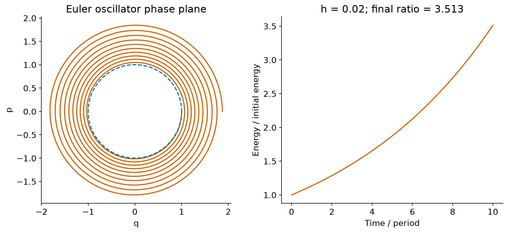
Euler's oscillator trajectory spirals outward and its energy grows to about 3.51 times its initial value. — Figure 2:The dimensionless oscillator uses $\omega=1$ , $h=0.02$ , and 3142 steps (approximately ten periods). Left: Euler expands the scaled phase-plane trajectory relative to the exact unit circle. Right: the exact discrete energy factor compounds to about 3.51. This is an oscillator diagnostic, not a computed spatial orbit in an inverse-square force.

Why Euler Fails: The Geometric View¶

Phase space: The space of all possible states, with position and momentum coordinates. Trajectories follow energy contours.

Liouville’s theorem: Phase space volume must be preserved in Hamiltonian systems

In scaled phase coordinates $(x,v/\omega)$ , the harmonic oscillator traces a circle; in unscaled position-velocity coordinates it generally traces an ellipse. Each Euler step moves along the tangent to the circle, placing the new point slightly outside. The phase space area increases, violating Liouville’s theorem that phase space volume must be preserved in Hamiltonian systems.

The Phase Error Problem¶

Energy and phase diagnose different errors. In scaled coordinates, one Euler step rotates by $\arctan(\omega h)$ while expanding the radius. Therefore

\omega_{\rm num}=\frac{\arctan(\omega h)}h =\omega-\frac{\omega^3h^2}{3}+O(h^4).

(21)

After $N=T/h$ steps, the unwrapped phase discrepancy is

\Delta\phi=T(\omega_{\rm num}-\omega) =-\frac{T\omega^3h^2}{3}+O(Th^4).

(22)

At fixed duration the oscillator’s phase error is second order even though Euler’s overall state error is first order: amplitude growth dominates the state error. At fixed $h$ , the phase lag accumulates linearly with time. This special diagnostic order does not make Euler a second-order integrator.

Predict: when $h$ is halved at fixed $T$ , should the leading energy error halve or quarter? What about the phase error?

import numpy as np
T = 2 * np.pi  # One period, with omega = 1 in dimensionless time.
for n in (100, 200, 400):
    h = T / n
    energy_error = np.expm1(n * np.log1p(h*h))
    phase_error = n * np.arctan(h) - T
    print(f"n={n}: relative energy error={energy_error:.5e}, "
          f"phase lag={phase_error:.5e} rad")

n=100: relative energy error=4.82911e-01, phase lag=-8.24881e-03 rad
n=200: relative energy error=2.18103e-01, phase lag=-2.06586e-03 rad
n=400: relative energy error=1.03717e-01, phase lag=-5.16695e-04 rad

Answer: two diagnostics, two orders

The energy error approaches first-order scaling; the phase lag approaches second-order scaling. Measure both at the same final time. Counting steps as oscillations would insert an extra factor of $1/h$ and give the wrong phase order.

When Does Euler Work?¶

Despite these failures, Euler has legitimate uses:

Very short integrations where $N(\omega h)^2 \ll 1$ for this oscillator
Resolved dissipative systems where the step also satisfies the stability limit; stiffness can make explicit Euler impractical
Quick explorations before using better methods
Teaching why better methods are needed!

The Fundamental Lesson¶

Euler’s method reveals a profound truth about numerical integration:

Local accuracy does not guarantee global stability

Euler has a second-order one-step defect ( $O(h^2)$ ) and first-order global error, yet it systematically violates conservation laws. This isn’t a bug — it’s a fundamental property of the discretization.

The tangent line approximation, while locally accurate, doesn’t respect the curved geometry of phase space. Each step compounds this geometric error until the qualitative behavior is wrong.

Answers and reasoning

There are $O(1/h)$ one-step defects over a fixed interval; their propagation through a Lipschitz right-hand side gives an $O(h)$ global bound.
Explicit Euler with negative $h$ still has oscillator energy factor $1+(\omega h)^2>1$ . It expands in either direction; a negative explicit step is not the inverse of a positive one.
After $N=T/|h|$ steps, assuming that is an integer, the phase-plane radius grows by $[1+(\omega h)^2]^{N/2}$ . This is the oscillator result, not a Kepler radius law.
At fixed finite duration, refinement can meet a target. It never creates a stable nonzero Euler step for the undamped oscillator, and its cost can become prohibitive.
The oscillator Jacobian determinant is $1+(\omega h)^2$ , so phase-space area expands by that factor each step.

Bridge to Part 2: The Quest for Better Methods¶

Euler’s catastrophic failure motivates our search for better integration methods. The failure isn’t just about accuracy — it’s about systematic bias. Every Euler step pushes slightly outward from the true trajectory. This accumulation of geometric errors destroys the physics we’re trying to simulate.

What we need are methods that:

Sample the derivative at multiple points to cancel biases
Achieve higher-order accuracy to reduce error accumulation
Maintain stability over long integration times
Preserve conservation laws or at least bound their violation

In Part 2, we’ll explore the Runge-Kutta family — methods that evaluate the derivative at carefully chosen intermediate points to achieve higher accuracy. By sampling the “curvature” of the solution, these methods can follow the true trajectory more faithfully. But as we’ll discover, even fourth-order accuracy isn’t enough to preserve energy over cosmic timescales.

The journey from Euler to modern integration methods is a journey from naive approximation to deep understanding of geometric structure. Each method we develop addresses specific failures of its predecessors, leading ultimately to symplectic integrators that preserve the fundamental geometry of physics.

Next: Part 2 - Building Better Methods