Learning Objectives
By the end of this section, you will be able to:
Derive explicit midpoint RK2 and explain the stage dependencies of RK4
Use the mathematical specification to write and verify your own RK implementations
Connect RK weights to quadrature rules from Module 2
Trace adaptive step acceptance and rejection using a worked Euler example
Analyze when higher-order methods help vs harm
Choose appropriate RK methods based on problem requirements
The Key Insight: Sample Multiple Points
Euler extends the initial tangent through the step. Curvature introduces a one-step defect, which motivates sampling additional slopes. Runge-Kutta methods evaluate the derivative at carefully chosen intermediate points, then combine these samples with specific weights to achieve higher-order accuracy.
This connects to quadrature from Module 2: We’re essentially performing numerical integration on:
But now the integrand depends on the unknown solution itself, requiring us to estimate intermediate values.
RK2 - The Midpoint Method
Geometric Intuition
Instead of blindly following the tangent from the starting point, we:
Take a half-step using the initial derivative
Evaluate the derivative at this midpoint
Use this midpoint derivative for the full step
This is analogous to the midpoint rule for integration, which we know from Module 2 is second-order accurate!
Complete Mathematical Formulation
Predictor-corrector method: A two-stage process where an initial estimate (predictor) is refined using better information (corrector).
The RK2 midpoint method is a predictor-corrector method:
Stage 1 - Predictor:
Stage 2 - Corrector:
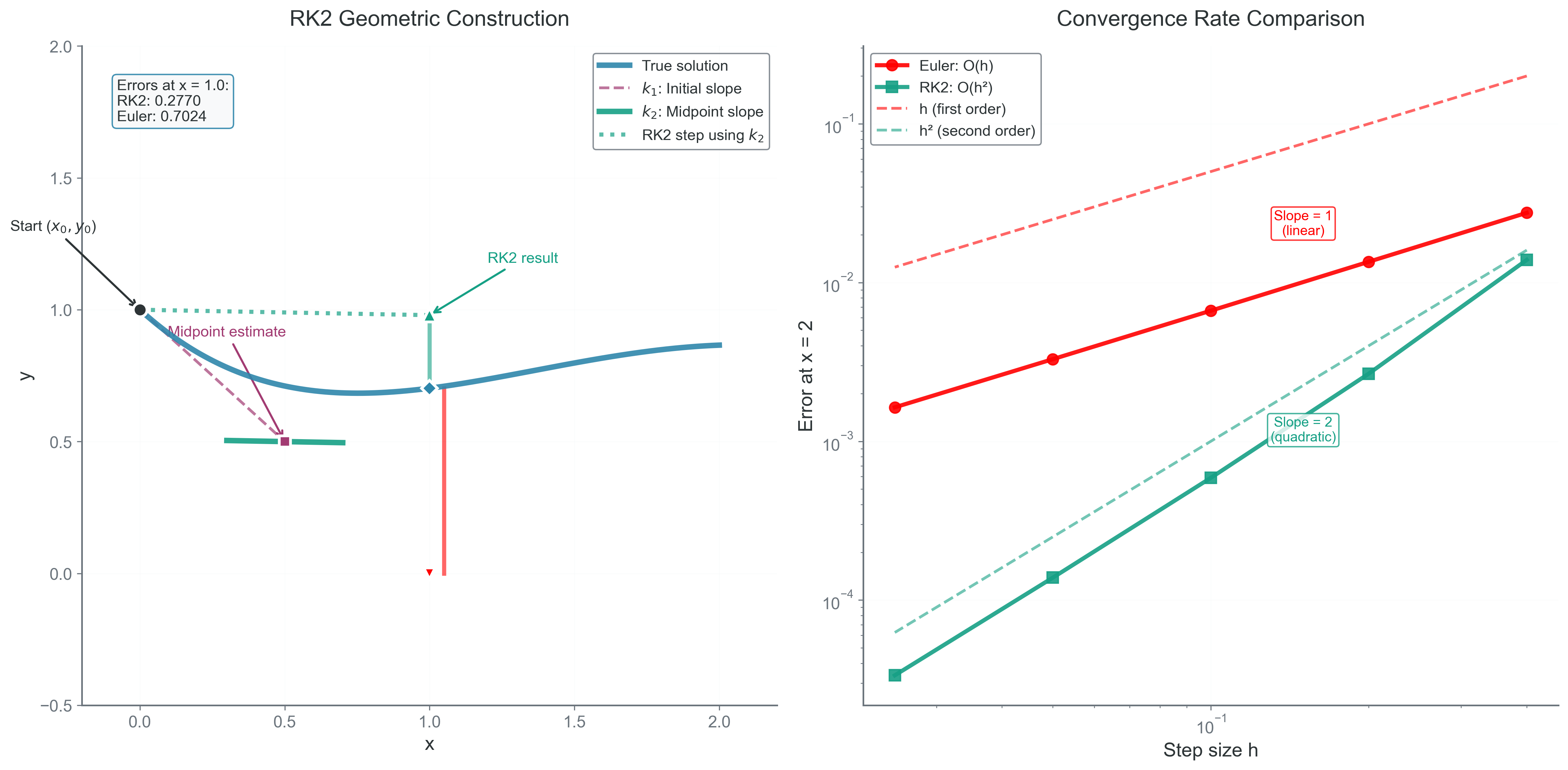
Figure 1:This dimensionless example solves , , with exact reference (the figure labels the independent variable ). In the left panel, : the initial slope predicts the midpoint state, and the slope at that predicted state advances the full step. Its absolute error is about 0.2770, versus Euler’s 0.7024; this coarse step is still inaccurate. The right panel compares errors at the fixed endpoint as decreases. The asymptotic trends approach first order for Euler and second order for midpoint RK2.
Error Analysis via Taylor Series
Differentiate the ODE along its solution. For a vector state, let be the state Jacobian. Then
so the exact solution begins
Try two stages, with and , and an update . A multivariate expansion gives
and the resulting update is
Matching the independent terms requires
Choose . Then and , giving the explicit midpoint formulas above. The midpoint slope consequently satisfies
Another choice, and , gives Heun’s explicit trapezoidal method. Both are second-order RK methods, but their intermediate states differ. This reading uses explicit midpoint when it says RK2. On a linear autonomous system they have the same one-step map; a nonlinear test can separate them. For , , their one-step values are and , respectively. Neither cubic coefficient matches the exact local expansion of ; both methods match through second order. Do not mix their stages and weights.
The RK2 update matches the true solution through :
Local truncation error:
Global error:
In a resolved truncation regime at fixed duration, halving the timestep reduces the leading global error by approximately four.
From mathematics to your implementation
The stage equations are the specification you will translate into Python. Write the RK2 and RK4 implementations yourself. We will use complete Euler examples to demonstrate array handling, stepping, and diagnostics; a working RK routine is not supplied here.
For Python, use independent variable first: f(t, state) returns the rate
of change of the NumPy-array state. In the equations above, denotes that
state; it can have several components. Addition and scalar multiplication then
operate on the entire array. The stage slopes must have the same shape as the
state. Their units are state units divided by time units; multiplying a slope
by gives a state increment.
Separate two responsibilities:
| Responsibility | Inputs | Output | What to establish |
|---|---|---|---|
| One step | A derivative callable, starting time and state, and a step length | A new state | Stage times, stage states, weights, shape, and no mutation of the supplied state |
| Repeated steps | A step routine and an integration interval | The endpoint or a recorded trajectory, as the caller needs | Endpoint handling, time bookkeeping, and where samples are stored |
First explain the method in mathematical statements, then write your own code. Before writing the loop, answer: which quantities belong to the original state, and which belong to a temporary stage? If a stage accidentally overwrites the starting state, later formulas describe a different method.
Do not judge correctness from a smooth-looking trajectory alone. A constant right-hand side checks basic increments. A time-dependent right-hand side tests whether stage times are used. A nonlinear state-dependent right-hand side tests whether intermediate states are used. Refinement over a fixed interval then checks the claimed global order. These checks probe different mistakes; none is a replacement for deriving the update.
Check the units and the meaning of a stage
In this reading, is a slope, not a step increment. It has the units of . Each predicted state therefore includes a factor of , and the final weighted sum includes one factor of . Some books define instead; copying one convention’s stage formulas into the other’s final update introduces an extra or missing factor of .
The midpoint state is a prediction used to evaluate a slope. It is not a second initial condition or a replacement for the starting state. Keeping those roles separate is part of the implementation work.
RK4 - The Classical Workhorse
Runge-Kutta 4 (RK4): A classical explicit method with four derivative evaluations per step and fourth-order global accuracy under its smoothness and stability assumptions.
RK4 samples the derivative at four carefully chosen points:
Stage 1: (derivative at start)
Stage 2: (derivative at midpoint using )
Stage 3: (derivative at midpoint using )
Stage 4: (derivative at endpoint using )
Final update:
The Connection to Simpson’s Rule
For a time-only right-hand side , the two midpoint evaluations are identical. The RK4 update then becomes
which is exactly Simpson quadrature over the time interval. Euler similarly reduces to left rectangles and explicit midpoint RK2 to midpoint quadrature.
For , however, and generally differ: they evaluate different predicted states at the same time. Simpson’s weights alone do not establish fourth-order ODE accuracy. The stage locations and dependencies must satisfy additional order conditions involving state derivatives of .
Check: for , start at , with . Then , , , and . The unequal midpoint slopes are precisely what the state-dependent problem adds to the quadrature analogy.
Error Analysis
Through Taylor series expansion to fourth order:
Local truncation error:
Global error:
In a resolved truncation regime at fixed duration, halving the timestep reduces the leading global error by approximately sixteen.
The General Runge-Kutta Framework
Butcher tableau: A compact notation for Runge-Kutta methods invented by John Butcher (1964), organizing the coefficients that define each method.
All explicit RK methods follow this pattern:
The coefficients define the method and are displayed in a Butcher tableau:
c₁ |
c₂ | a₂₁
c₃ | a₃₁ a₃₂
⋮  | ⋮
cₛ | aₛ₁ aₛ₂ ... aₛ,ₛ₋₁
---|--------------------
   | b₁  b₂  ...  bₛ
For RK4:
0   |
1/2 | 1/2
1/2 | 0   1/2
1   | 0   0   1
----|----------------
    | 1/6 2/6 2/6 1/6
Follow the dependencies, not just the weights
The two midpoint stages occur at the same time but generally at different predicted states. The second midpoint evaluation revises the slope information used to predict the endpoint.
Every stage state in the formulas is built from the original plus a specified increment. The arrows show dependencies; they do not mean that stage states are advanced sequentially by a full ODE step. The two midpoint states are generally not points on the exact trajectory either.
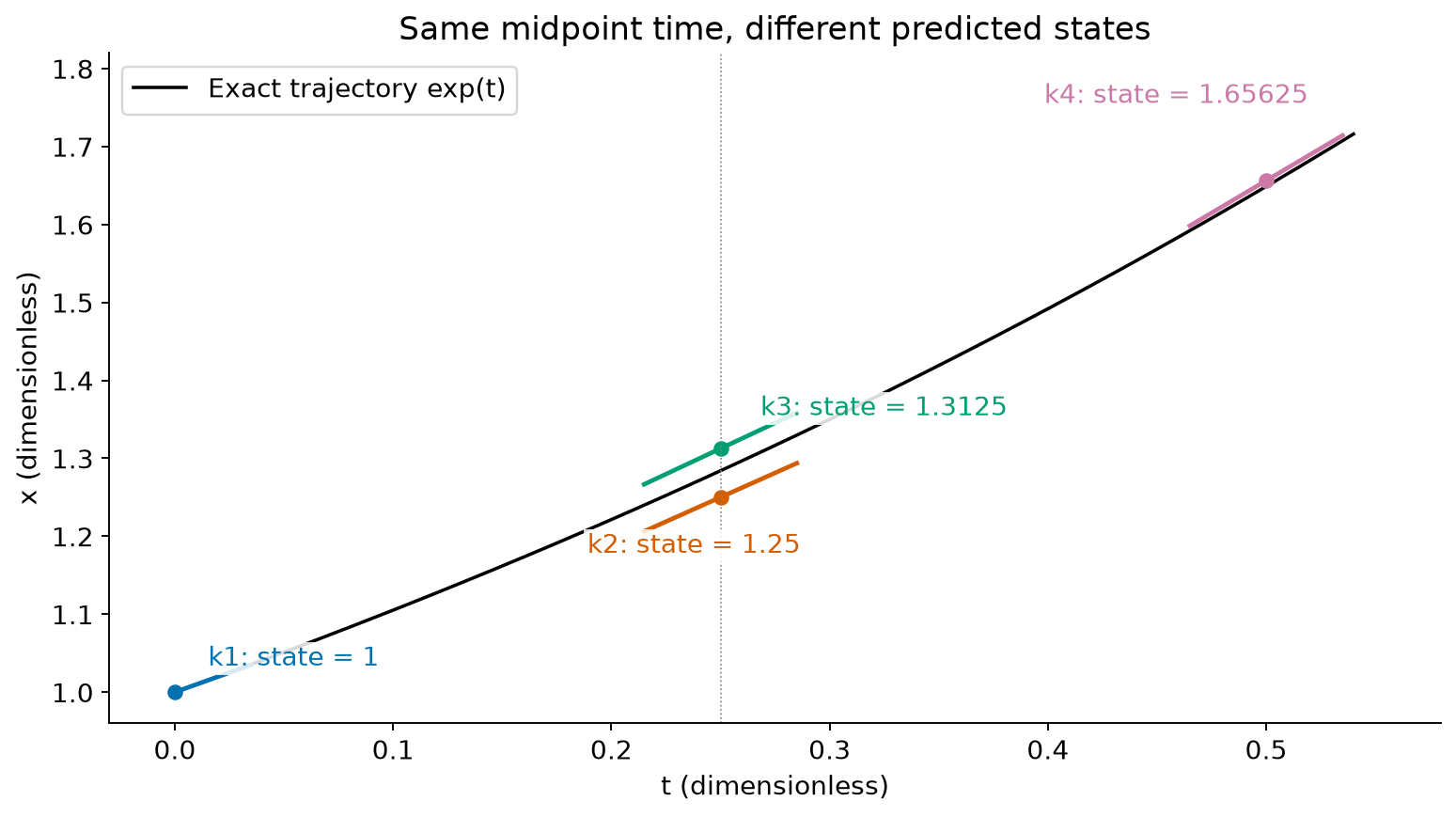
Figure 2:For , , and , the midpoint predictions are 1.25 and 1.3125, whereas the exact midpoint value is . RK4 uses information from approximate stage states to construct an accurate endpoint; it does not require every intermediate state to have fourth-order accuracy.
Optional derivation: where fourth order comes from
The scalar exponential test is useful, but it cannot test all the terms that occur in a nonlinear system. To see the missing terms, consider an autonomous vector equation . A time-dependent problem fits this form after adding time as a state component: .
Write for the Jacobian, for the second derivative applied to two vectors, and for the third derivative applied to three. All quantities below are evaluated at the starting state. Repeated application of the chain rule gives
These are distinct ways that the vector field can vary along a solution. For example, differentiating changes both and , which produces the two terms in . In a linear problem, and vanish. That is why a linear convergence test alone cannot establish general nonlinear fourth order.
The stage/tableau formulation is also described in Butcher’s introduction to practical Runge–Kutta methods, Section 3. Here we work out the matching conditions needed for this reading.
Let , , and be the tableau coefficients. Superscripts on in the table mean componentwise powers, and . Expanding the stage equations and matching each coefficient in gives:
| Term in the solution expansion | Required condition |
|---|---|
The factors are not all : the stage expansion itself supplies factorials and multiplicities. For instance, its coefficient of is , which must equal .
For the classical RK4 tableau, and . Two checks illustrate the calculation:
The conditions involving are what a list of quadrature weights leaves out. Verify one fourth-order condition by hand before checking the result below.
Check a fourth-order condition
, so . Also, and give and , respectively. These checks supplement the quadrature-like conditions; they do not replace them.
Under sufficient smoothness, these conditions give a one-step defect of . Propagation over a fixed interval, with the appropriate stability and regularity assumptions, gives global error. This is the mathematical claim to test with your implementation, not an assurance that every plot of error versus step length will have slope four.
Adaptive Timestep Control
Real problems have varying timescales. When a planet is far from the sun, we can take large steps. During close encounters, we need tiny steps. Adaptive methods adjust dynamically.
The Embedded Runge-Kutta Approach
The idea: compute two different order estimates using the same function evaluations, then use their difference to estimate error.
An embedded example: Fehlberg 4(5)
The original six-stage Fehlberg pair computes both fourth- and fifth-order solutions. The name RK45 is also used for other pairs: SciPy uses Dormand–Prince, not these six stages. For the Fehlberg example:
Compute six values (shared between both estimates)
Combine with 4th-order weights
Combine with 5th-order weights
Error estimate:
Suggested next timestep (with a safety factor):
For vectors, first scale each component by an allowance such as atol + rtol * abs(reference_state) and use a stated norm. Bound the step-growth factor and handle a zero estimate explicitly. If the scaled estimate is acceptable, accept the step and continue. Otherwise, reject and retry with smaller .
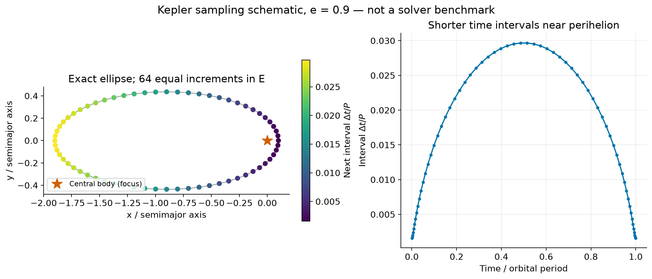
Figure 3:This is a kinematic sampling schematic, not an adaptive-solver benchmark. The exact Kepler ellipse has eccentricity and is sampled at 64 equal increments of eccentric anomaly . Kepler’s relation gives the time of each point. The left panel colors each point by the following time interval; the right plots those intervals against their time midpoints. This illustrates why the rapid motion near perihelion calls for finer time resolution. It makes no accuracy or efficiency claim; the executable Euler experiment below demonstrates an actual error-controlled acceptance rule.
Watch an adaptive controller make a decision
We can study acceptance and rejection using Euler steps, while leaving the RK implementations to you. Consider the dimensionless decay problem , , with exact solution . It gives us a reference for checking the numerical experiment without introducing another physical model.
Take one Euler step of length and, separately, two Euler steps of length , both starting from the same . If the leading one-step defect is , the two-half-step result has approximately half the defect of the coarse result. Their difference therefore estimates the two-half-step local error in the smooth, small-step regime:
This is still a first-order method. We accept itself; we do not apply an extrapolation correction. The comparison estimates a local error and does not reveal the exact accumulated error of the trajectory.
For this example, define the scale and normalized estimate explicitly:
Accept when . Rejection leaves both the accepted time and accepted state unchanged. The proposed next step uses because this estimator scales as . The exponent would change for another estimator. Growth limits and a safety factor make the controller less abrupt; they do not turn an estimate into a mathematical bound.
Predict before running: Will the initial step of length 1 be accepted? When the solution becomes small, which part of the allowance will eventually matter more? Does every accepted step imply that the final solution is within one tolerance of the exact answer?
import numpy as np
import matplotlib.pyplot as plt


def euler_trial(f, t, u, h):
    """Compare one Euler step with two Euler half-steps; scalar state."""
    coarse = u + h*f(t, u)
    half = u + (h/2)*f(t, u)
    fine = half + (h/2)*f(t + h/2, half)
    return fine, abs(fine-coarse)


def adaptive_euler_decay(rtol, atol, initial_h=1.0, end_time=4.0):
    """A teaching controller for u'=-u; accepts the two-half-step state."""
    if not np.all(np.isfinite([rtol, atol, initial_h, end_time])):
        raise ValueError("Parameters must be finite")
    if rtol < 0 or atol <= 0 or initial_h <= 0 or end_time <= 0:
        raise ValueError("Require rtol >= 0 and positive atol, step, and end time")
    t, u, h = 0.0, 1.0, initial_h
    times, values, trials = [t], [u], []
    for attempt in range(10000):
        if t >= end_time:
            return np.array(times), np.array(values), np.array(trials)
        h = min(h, end_time-t)  # Land on the requested final time.
        if t + h == t:
            raise RuntimeError("The proposed step cannot advance floating-point time")
        fine, estimate = euler_trial(lambda time, value: -value, t, u, h)
        scale = atol + rtol*max(abs(u), abs(fine))
        ratio = estimate/scale
        if not np.isfinite(ratio):
            raise RuntimeError("Non-finite error estimate")
        accepted = ratio <= 1.0
        trials.append((t, h, ratio, accepted))
        if accepted:
            t, u = t+h, fine
            times.append(t)
            values.append(u)
        # Zero estimated error permits bounded growth, not an infinite step.
        factor = 2.0 if ratio == 0 else np.clip(0.9*ratio**(-0.5), 0.2, 2.0)
        h *= factor
    raise RuntimeError("Attempt limit reached")


adaptive_t, adaptive_u, adaptive_trials = adaptive_euler_decay(1e-3, 1e-5)
print("  start t    trial h    scaled estimate   accept?")
for t, h, ratio, accepted in adaptive_trials[:6]:
    print(f"{t:9.4f}  {h:9.4f}  {ratio:15.4f}   {bool(accepted)}")
print("Final actual absolute error:", abs(adaptive_u[-1]-np.exp(-adaptive_t[-1])))
start t trial h scaled estimate accept?
0.0000 1.0000 247.5248 False
0.0000 0.2000 9.9010 False
0.0000 0.0572 0.8100 True
0.0572 0.0572 0.8095 True
0.1144 0.0572 0.8095 True
0.1716 0.0572 0.8095 True
Final actual absolute error: 0.0010884703398220882
The first three statements in euler_trial are exactly Euler updates. This
transparent version evaluates the starting derivative twice; caching it would
save one call per trial, without changing the method. The controller records
rejected trials as well as accepted ones, so the work cannot be inferred just
from the number of stored solution points.
accepted_trials = adaptive_trials[:, 3].astype(bool)
fig, axes = plt.subplots(2, 1, figsize=(8, 6), layout="constrained")
axes[0].plot(adaptive_t, adaptive_u, label="accepted Euler half-steps")
axes[0].plot(adaptive_t, np.exp(-adaptive_t), "--", label="exact decay")
axes[0].set(xlabel="dimensionless time", ylabel="dimensionless u")
axes[0].legend()
for mask, label, marker in ((accepted_trials, "accepted", "o"),
                            (~accepted_trials, "rejected", "x")):
    axes[1].semilogy(adaptive_trials[mask, 0], adaptive_trials[mask, 1],
                     marker, ms=4, label=label)
axes[1].set(xlabel="start time of trial", ylabel="trial step length")
axes[1].legend()
plt.show()

for requested_rtol in (1e-2, 1e-3, 1e-4):
    ts, us, trials = adaptive_euler_decay(requested_rtol, 1e-5)
    actual = abs(us[-1]-np.exp(-ts[-1]))
    final_allowance = 1e-5 + requested_rtol*abs(us[-1])
    print(f"rtol={requested_rtol:.0e}: accepted={len(ts)-1}, attempts={len(trials)}, "
          f"final error={actual:.3e}, error/final allowance={actual/final_allowance:.2f}")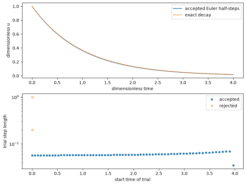
rtol=1e-02: accepted=22, attempts=23, final error=3.226e-03, error/final allowance=20.05
rtol=1e-03: accepted=67, attempts=69, final error=1.088e-03, error/final allowance=39.98
rtol=1e-04: accepted=163, attempts=166, final error=4.780e-04, error/final allowance=40.57
Explain the controller’s evidence
At the first trial, Euler gives and the two half-steps give . The discrepancy is much larger than the allowance , so the controller rejects the step. Repeated rows with the same starting time show retries, not repeated advancement of the solution.
While dominates, an approximately constant relative decay rate leads to roughly constant accepted steps. As becomes smaller, the absolute allowance becomes more influential. Extending the end time makes that transition easier to observe; decreasing does not create unlimited information about its relative accuracy.
The printed final error can exceed the allowance used for an individual step. Local defects accumulate and propagate. Tighter tolerances should be tested against the actual quantity of interest under refinement; the solver’s acceptance decision alone does not certify a final-time error target.
For a new problem without an exact solution, compare tolerances and another justified diagnostic. The exact decay here lets us test that reasoning before using it in a harder setting.
The same controller logic can use an embedded RK error estimate, with the appropriate estimator order and vector scaling. Constructing the RK stages remains your work. A request for evenly spaced output is also different from a request for evenly spaced internal steps: established libraries can interpolate between accepted steps. SciPy’s solver documentation distinguishes these roles and describes component-dependent absolute tolerances.
When to Use Adaptive Methods
Good for:
Problems with varying timescales
Unknown dynamics
Achieving specified accuracy efficiently
Initial exploration of new systems
Bad for:
Long-term Hamiltonian systems when ordinary state-dependent step selection would compromise a fixed-step symplectic method
Parallel simulations (variable timesteps complicate synchronization)
Compare accuracy and work with a defined benchmark
A comparison needs a defined system, initial state, duration, step size, error metric, and cost metric. We use the dimensionless simple harmonic oscillator (SHO), , , with . Its exact solution is and its period is .
The reference plots below retain the comparisons among Euler, explicit midpoint RK2, classical RK4, and kick–drift–kick leapfrog. The figures were generated separately; no RK implementation is supplied in the page or an accompanying notebook. Use the mathematics to construct your own methods, and use the observables to decide what your implementation needs to establish.
One oscillator, four diagnostics
Each method uses 100 steps per period for 20 periods. Before examining the figure, predict which method increases energy, which damps it, and whether bounded energy guarantees accurate phase. The inset enlarges the trajectories near the unit circle; Euler’s growth would otherwise hide their differences.
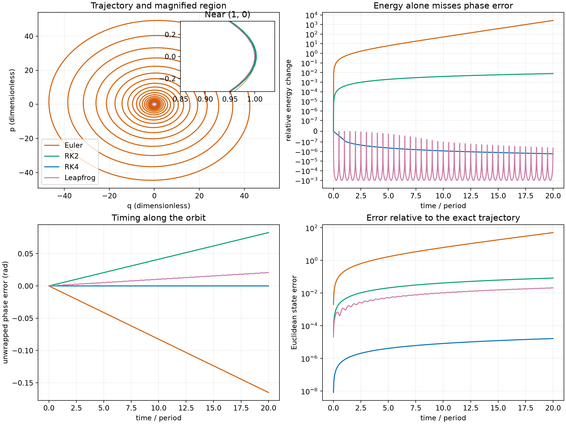
Figure 4:At the same step length, the four methods differ in amplitude, phase, and state error. These are reference calculations for the stated linear oscillator, not a claim that one method wins for every equation or duration. The energy axis uses a symmetric logarithmic scale so small damping and large growth can both be seen. The inset resolves trajectories near the exact unit circle.
For this oscillator, the diagnostic definitions are
The phase error is . Unwrapping chooses a continuous branch by removing jumps; it requires sufficiently resolved phase advances. At this resolution, that assumption holds. A point close to the unit circle can still be at the wrong angle, so energy agreement alone is incomplete.
Tools for inspecting a trajectory
These diagnostics consume a trajectory; they do not construct RK stages. The next cell demonstrates them using a complete Euler calculation. The state has two dimensionless components; a physical state with mixed units would need specified component scales before taking a combined norm.
def euler_sho(steps_per_period=100, periods=20):
    """A complete Euler example; returns times and two-component states."""
    if any(isinstance(value, (bool, np.bool_)) or not isinstance(value, (int, np.integer))
           or value <= 0 for value in (steps_per_period, periods)):
        raise ValueError("Use positive integer step and period counts")
    n = steps_per_period*periods
    h = 2*np.pi/steps_per_period
    times = h*np.arange(n+1)
    states = np.empty((n+1, 2))
    states[0] = [1.0, 0.0]
    for i in range(n):
        q, p = states[i]  # Both derivatives use the old state.
        states[i+1] = states[i] + h*np.array([p, -q])
    return times, states


def sho_diagnostics(times, states):
    """Measure energy, phase, and Euclidean state error for omega=1."""
    times = np.asarray(times, dtype=float)
    states = np.asarray(states, dtype=float)
    if times.ndim != 1 or states.shape != (len(times), 2):
        raise ValueError("Expected times (n,) and states (n, 2)")
    if not np.all(np.isfinite(times)) or not np.all(np.isfinite(states)):
        raise ValueError("Diagnostics require finite data")
    energy = np.sum(states**2, axis=1)/2
    phase = np.unwrap(np.arctan2(-states[:, 1], states[:, 0]))
    exact = np.column_stack((np.cos(times), -np.sin(times)))
    state_error = np.linalg.norm(states-exact, axis=1)
    return energy, phase-times, state_error


euler_times, euler_states = euler_sho()
euler_energy, euler_phase_error, euler_state_error = sho_diagnostics(euler_times, euler_states)
print("Euler maximum state error:", euler_state_error.max())
print("Euler final relative energy change:", euler_energy[-1]/euler_energy[0]-1)
print("Euler final phase error (rad):", euler_phase_error[-1])
Euler maximum state error: 50.43601922172834
Euler final relative energy change: 2643.2399896798
Euler final phase error (rad): -0.16497620494871512
Apply the definitions to another trajectory only after checking its equations, initial condition, time units, and state ordering. The helper’s exact reference is specific to this SHO setup. A plausible output from a helper used on the wrong problem is not a validation.
| Method | Derivative evaluations per step | What is counted? |
|---|---|---|
| Euler | 1 | Full oscillator right-hand side |
| Explicit midpoint RK2 | 2 | Full right-hand side |
| Classical RK4 | 4 | Full right-hand side |
| Leapfrog | 2 without reuse | Force evaluations; retaining the final force can reduce later steps to 1 new call |
Each trajectory has 2000 steps. A force evaluation and a full right-hand-side call need not have equal cost in an application. These counts are not timings. To compare efficiency, select the observable, duration, and error requirement first, then compare work needed to meet that same requirement. Formal order alone does not determine a universal crossover accuracy.
Answer: interpret the diagnostics together
Euler grows in amplitude; explicit midpoint RK2 also injects energy but much more slowly here. RK4 damps slightly. Leapfrog’s energy oscillates in a bounded band at this stable step, while its phase still drifts. The state-error panel combines discrepancies that an energy-only diagnostic can miss.
Halving the step at fixed duration tests the expected orders. Increasing the duration tests a different question: the accumulated error over the time span we care about. A method can pass one experiment and miss the requirement in the other. The axes and the comparison must state which question is being asked.
Why high order does not imply energy conservation
For the oscillator, put . The explicit RK stability function determines the energy factor per step. Euler gives ; explicit midpoint gives ; classical RK4 gives
Thus RK4 damps this oscillator for , while Euler and RK2 increase its energy. Neither the direction nor the size of a Kepler-orbit energy drift follows from this linear calculation. RK4 is globally fourth order and has an one-step defect; those orders say how state error scales at fixed duration, not that a conserved quantity remains exact.
The explicit RK methods discussed here are not symplectic for general Hamiltonian systems. Some implicit RK methods are symplectic, so this is not a defect of every Runge–Kutta method. A measured energy drift, the Jacobian’s volume change, and the full symplectic condition are related diagnostics, but one does not substitute for the others.
Answers and reasoning
The predicted midpoint state provides a slope whose update matches the solution through second order; using an endpoint slope requires different weights to obtain a second-order method.
For , the two midpoint slopes coincide and RK4 reduces exactly to Simpson. State-dependent problems need the stage order conditions too.
Adaptation helps resolve changing timescales. Ordinary state-dependent step selection can compromise the geometric argument for fixed-step symplectic integration; uniform output times alone do not forbid adaptive internal steps.
A high Taylor order reduces finite-time truncation error but does not impose an exact conservation identity.
Classical RK4 uses four right-hand-side evaluations per step.
On the oscillator, the real two-dimensional map has area factor . It contracts inside the stated RK4 stable interval, consistent with the observed damping.
Bridge to Part 3: The Need for Geometric Integration
The Runge–Kutta family improves finite-time state accuracy by evaluating the derivative at carefully chosen stages. For a short trajectory calculation, adaptive RK can be an excellent choice. For long autonomous Hamiltonian integrations, geometric preservation supplies a different source of control.
In Part 3, we will derive leapfrog and ask exactly what its geometry preserves. Second-order leapfrog does not automatically beat fourth-order RK4: the answer depends on the observable, duration, resolution, and cost. Energy can remain well behaved while orbital phase becomes inaccurate. The comparison experiment keeps these diagnostics separate so you can justify a method choice.
Next: Part 3 - Symplectic Integration