Learning Objectives
By the end of this section, you will be able to:
Analyze stability regions for different integration methods
Diagnose and handle stiff equations
Predict when numerical methods will become unstable
Choose appropriate methods based on stability requirements
Implement implicit methods for challenging problems
Linear Stability Theory
To understand when methods fail catastrophically, we analyze their behavior on the test equation:
where . The true solution is .
Stability function: The amplification factor relating consecutive numerical solution values: .
When we apply a numerical method, we get:
where is the stability function with .
Stability region: The set of complex values for which , ensuring bounded solutions.
For bounded solutions, we need . The stability region is the set of values where this holds.
Stability Functions for Common Methods
Let’s derive the stability functions for our methods:
Euler’s Method
Applying Euler to :
Therefore:
This is stable when , which defines a circle of radius 1 centered at .
RK2 (Midpoint)
Following through the RK2 steps:
Therefore:
RK4
Through similar analysis (but more algebra):
For this linear test equation, it is exactly the degree-four Taylor polynomial of . That does not make the general state-dependent RK4 update a scalar exponential polynomial.
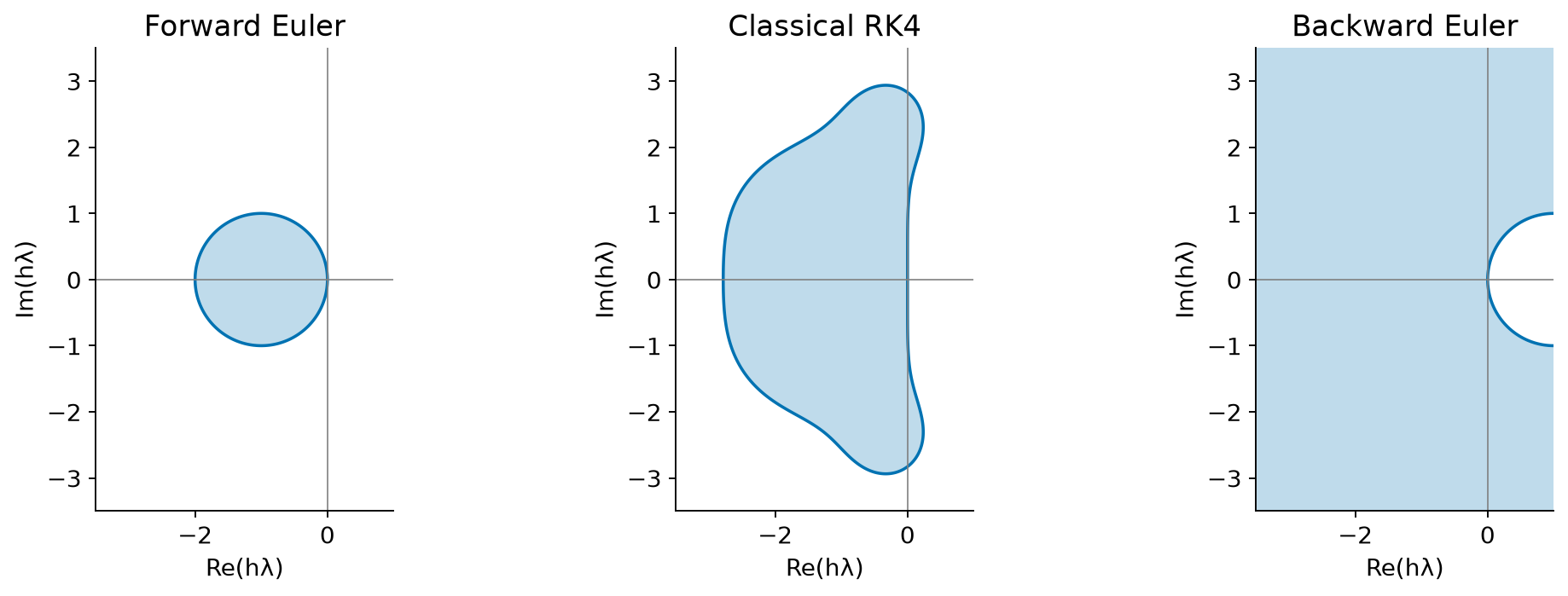
Shading marks for the scalar test equation. Forward Euler’s region touches the imaginary axis only at zero. Backward Euler covers the left half-plane but can still introduce substantial artificial damping.
Physical Interpretation
For different types of problems, we need different stability characteristics:
Oscillatory Systems (Circular Orbits)
For a harmonic oscillator with frequency :
Eigenvalues: (purely imaginary)
Stability requires the particular points to lie in the method’s stable set
Euler: Unstable for every , since ; it amplifies the oscillator
RK4: Stable on this linear oscillator for ; generally damps inside that interval
Leapfrog: Stable for with no damping!
Dissipative Systems (Damped Motion)
For exponential decay with rate :
Eigenvalue: (negative real)
Stability requires the particular negative-real point in the stability region
Euler: Stable for
RK4: Stable for
Stiff Equations - When Stability Dominates
Stiff equation: An ODE where stability requirements force much smaller timesteps than accuracy requirements. Named because they arise in stiff mechanical systems.
What Makes an Equation Stiff?
Widely separated timescales are a common source of stiffness, not a necessary definition. After fast transients decay, we may be tracking slow evolution while an explicit method still requires tiny timesteps for stability. The comparison is between the step needed for accuracy on the interval of interest and the step allowed by the chosen method’s stability region.
Understanding Stiffness Through Examples
Example 1: Chemical Kinetics
Consider a reaction where species A slowly converts to B, but B rapidly equilibrates:
The eigenvalues are (slow) and (fast).
The fast transient decays as ; after its amplitude is about of its initial value. For initial data and error targets that make this remnant negligible, then follows the slowly decaying . Forward Euler still needs to damp the fast numerical mode, even when the slow evolution could meet the accuracy target with a much larger step.
Example 2: Stellar Interior with Radiative Cooling
A thermal model can contain a cooling relaxation timescale much shorter than the duration of interest. For a stated toy model , linearization about gives
An explicit method may need to resolve this fast relaxation even while the equilibrium changes slowly. The law here is a pedagogical cooling model, not a universal prescription for stellar shocks; real cooling depends on opacity, density, ionization, and radiation transport.
Non-stiff equation: An ODE where accuracy requirements determine the timestep, with stability easily satisfied. Most orbital mechanics problems are non-stiff.
Non-Stiff vs Stiff: The Key Distinction
Non-stiff problems, for the chosen method and interval, allow accuracy to set the step without a much stricter stability restriction. Similar eigenvalue magnitudes are not a sufficient definition; even the scalar equation can be stiff over a long interval after its transient decays. Examples:
Planetary orbits (all periods within a few orders of magnitude)
Pendulum oscillations
Wave propagation in uniform media
Widely separated decay rates are one common source of stiffness. The timestep can be forced by stability of the fastest mode even after it has decayed; a scalar fast-decay problem can also be stiff over a long interval. Examples:
Chemical reaction networks
Radiative transfer with cooling
Electrical circuits with multiple timescales
Implicit Methods for Stiff Problems
Implicit method: A numerical scheme where the unknown appears on both sides of the equation, requiring solution of an algebraic system at each step.
Implicit methods evaluate the derivative at the future point, giving superior stability at the cost of solving equations.
Backward Euler
Instead of , we use:
This is implicit because appears on both sides!
Stability Analysis
For the test equation :
Stability function:
This is stable for the entire left half-plane! We call this A-stable.
A limiting check: for with , forward Euler’s factor is -9, while backward Euler’s is . The exact factor is . The implicit result is bounded and decays, but one step still does not resolve the actual fast transient accurately.
Solving the Implicit Equation
The challenge: we must solve for .
For nonlinear , this requires iteration. Newton’s method is typical:
import numpy as np

def backward_euler_step(y, t, h, f, df_dy, tol=1e-10):
    """
    Single backward Euler step
    Requires a one-dimensional state array and its square Jacobian df/dy.
    tol bounds the algebraic residual norm, not the time-integration error.
    """
    y = np.asarray(y, dtype=float)
    y_new = y.copy()  # Initial guess

    for _ in range(10):  # Newton iterations
        # Residual: R(y_new) = y_new - y - h*f(y_new, t+h)
        residual = y_new - y - h*f(y_new, t + h)

        if np.linalg.norm(residual) < tol:
            return y_new

        # Jacobian of residual
        J = np.eye(len(y)) - h*df_dy(y_new, t + h)

        # Newton update
        delta = np.linalg.solve(J, -residual)
        y_new = y_new + delta

    raise RuntimeError("Newton iteration failed to converge")
Implicit Midpoint Rule
A second-order implicit method:
Implicit midpoint is A-stable and symplectic for canonical Hamiltonian systems when the implicit solve is exact. It is not L-stable: its amplification tends to -1 for very stiff decay, so it can retain alternating unresolved transients. A-stability does not guarantee good damping or accuracy, and a loose nonlinear solve can spoil the structure.
The CFL Condition
CFL condition: Courant-Friedrichs-Lewy condition - the numerical domain of dependence must contain the physical one; its numerical coefficient depends on the scheme. Named after the mathematicians who discovered it in 1928.
The CFL condition is a necessary stability criterion for hyperbolic PDEs that also applies to ODEs from spatial discretization:
where is the spatial grid spacing, is the maximum wave speed, and depends on the spatial and temporal discretizations and dimension. A CFL bound alone is not a sufficient stability proof.
For the wave equation discretized in space:
Centered second differences in one dimension give frequencies up to .
Coupling that semidiscretization to leapfrog gives away from the boundary; coupling it to forward Euler remains unstable on the imaginary axis.
This means finer spatial grids require smaller timesteps!
Diagnosing Integration Problems
Systematic Debugging Approach
When your integration fails, follow this diagnostic sequence:
Check for NaN/Inf: Could indicate instability, an invalid function domain, division by zero, or overflow
Plot the solution: Look for oscillations growing exponentially
Compute eigenvalues: Estimate
Check stability region: Do all relevant complex values lie inside it? For non-normal systems, eigenvalues alone can miss transient amplification.
Test with smaller h: Does halving h fix the problem?
Monitor energy: For conservative systems, is energy bounded?
Stability Test Code
import numpy as np

def stability_test(method, lambda_val, h_values):
    """Flag non-finite or large finite-run outputs; not a stability proof."""
    results = []

    for h in h_values:
        y = 1.0  # Initial condition
        stable = True

        for n in range(1000):
            y = method(y, lambda_val, h)

            if not np.isfinite(y) or abs(y) > 1e10:  # Failure of this finite-run check
                stable = False
                break

        results.append((h, stable, abs(y)))

    return results
A True flag means only that this run stayed finite and below the stated
threshold for 1000 steps. Slow growth can pass that check. Use the analytical
condition for this test equation and report the finite-run
diagnostic separately. A nan result is always a failure of this check.
Answers and reasoning
Oscillatory linear modes have eigenvalues ; their amplification is tested at , not on the negative real axis.
Stiffness means stability forces steps much shorter than accuracy needs over the interval of interest, often after a fast transient has decayed.
Implicit steps require algebraic solves and do not remove accuracy requirements. Their damping can also distort oscillations.
Spatial discretization produces modes whose eigenvalues depend on grid spacing. The time integrator must stably advance those modes; the CFL coefficient depends on both discretizations.
Explicit steps are simpler and often cheaper individually; implicit steps can permit much larger stable advances on stiff problems but require reliable solves.
Strong numerical damping can erase an oscillation that the physical system preserves. Backward Euler is stable there but not necessarily accurate; boundedness alone is insufficient.
Bridge to the synthesis: choose and verify a method
Stability identifies restrictions that an error tolerance alone cannot enforce. The synthesis brings together step size, accuracy, conservation, and cost. Before optimizing a solver, establish a reference problem and a diagnostic that would reveal the failure mode you care about. A faster unstable solution is still an incorrect calculation; a stable result can still have unacceptable phase or trajectory error.
Next: Summary and Synthesis