Part 3: Symplectic Integration - Geometry Over Accuracy - COMP 521: Introduction to Scientific Computing and Data Science

Learning Objectives¶

By the end of this section, you will be able to:

Explain Hamiltonian mechanics and phase space structure
Prove symplecticity of leapfrog/Verlet methods
Understand modified Hamiltonians and bounded energy error
Implement symplectic integrators for conservative systems
Choose between accuracy and structure preservation

The Fundamental Insight¶

Symplectic integrator: A numerical method that preserves the symplectic structure (phase space volume and geometric properties) of Hamiltonian systems.

A symplectic integrator preserves the canonical two-form, a geometric constraint stronger than volume preservation in more than one degree of freedom. It still has truncation error: geometry and accuracy are both design criteria.

Symplectic maps preserve canonical phase-space volume in exact arithmetic.
A symmetric method such as fixed-step leapfrog is also time reversible; symplecticity alone does not imply reversibility.
Near-conservation of energy over long times needs smoothness, sufficiently small fixed steps, and a trajectory in a suitable bounded region.
Stability and accurate phase still need independent checks.

These distinctions let us ask a sharper question than “does it conserve physics?”: which property is exact for the discrete map, which is approximate, and over what regime have we checked it?

Hamiltonian Mechanics Refresher¶

Hamiltonian: A function $H(q,p,t)$ that represents the total energy of a system, where $q$ are generalized coordinates and $p$ are conjugate momenta.

Before diving into symplectic integration, let’s recall the Hamiltonian formulation of mechanics. For a system with positions $q$ and momenta $p$ , the Hamiltonian $H(q,p,t)$ represents total energy:

H(q,p) = T(p) + V(q)

(1)

where $T(p)$ is kinetic energy and $V(q)$ is potential energy.

For a particle of mass $m$ in potential $V(q)$ :

H = \frac{p^2}{2m} + V(q)

(2)

Hamilton’s equations govern the evolution:

\boxed{\frac{dq}{dt} = \frac{\partial H}{\partial p}, \quad \frac{dp}{dt} = -\frac{\partial H}{\partial q}}

(3)

These equations have remarkable properties:

Energy conservation: $\frac{dH}{dt} = 0$ for time-independent $H$
Phase space volume preservation: Liouville’s theorem
Symplectic structure: The flow preserves a geometric structure

The Phase Space Perspective¶

Phase space: The space of all possible states of a system, with position and momentum (or velocity) as coordinates.

In phase space, each point $(q,p)$ represents a complete state of the system. Trajectories follow contours of constant energy $H = E$ .

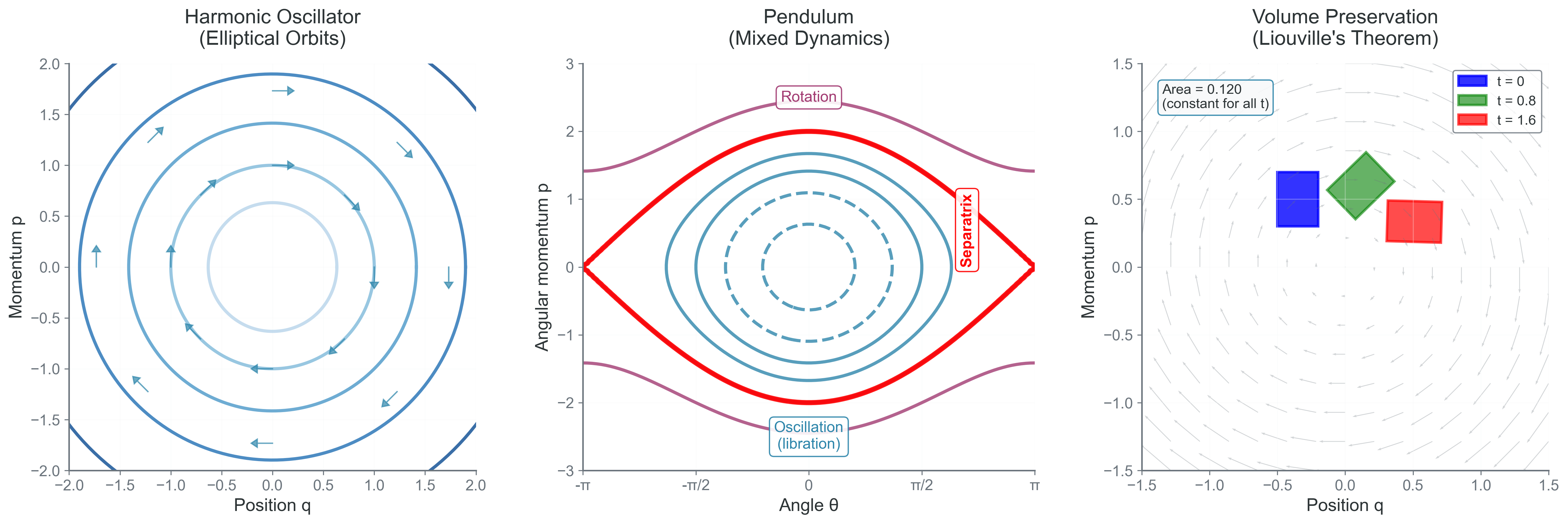
Oscillator and pendulum energy contours accompany equal-area phase-space regions deformed by Hamiltonian flow. — Figure 1:Phase space structure of Hamiltonian systems. (Left) Harmonic oscillator: closed orbits on energy surfaces. (Middle) Pendulum: separatrix divides oscillation from rotation. (Right) Liouville’s theorem: phase space volume is preserved under Hamiltonian flow—areas deform but don’t change size. This geometric structure is what symplectic integrators preserve, without by itself guaranteeing numerical stability for any step size.

Liouville’s Theorem¶

Liouville’s theorem: The phase space volume occupied by an ensemble of states is preserved under Hamiltonian evolution.

Liouville’s theorem states that phase space volume is preserved under Hamiltonian flow. Mathematically, for a volume element $dV = dq\,dp$ :

\frac{d(dV)}{dt} = 0

(4)

This is equivalent to saying the flow is incompressible. Standard numerical methods violate this theorem! They artificially compress or expand phase space, leading to systematic errors.

The Leapfrog/Verlet Method¶

The leapfrog method (also called Verlet or Störmer-Verlet) staggers position and velocity updates to preserve symplectic structure.

The Algorithm¶

For a Hamiltonian $H(q,p) = T(p) + V(q)$ where $T(p) = p^2/(2m)$ :

\boxed{ \begin{align} \text{Algorithm: Leapfrog Integration} \\ \hline &\text{Input: } q_n, p_n, h, \text{force function } F(q) = -\nabla V(q) \\ &\text{Step 1 (kick):} \quad p_{n+1/2} = p_n + \frac{h}{2}F(q_n) \\ &\text{Step 2 (drift):} \quad q_{n+1} = q_n + \frac{h}{m}p_{n+1/2} \\ &\text{Step 3 (kick):} \quad p_{n+1} = p_{n+1/2} + \frac{h}{2}F(q_{n+1}) \\ &\text{Output: } q_{n+1}, p_{n+1} \end{align} }

(5)

Why “Leapfrog”?¶

Positions and momenta “leapfrog” over each other in time:

Time:     t₀    t₁/₂    t₁    t₃/₂    t₂
          |      |      |      |      |
Position: q₀            q₁            q₂
Momentum:       p₁/₂          p₃/₂

The symplectic argument comes from composing the exact kick and drift flows, not from staggered storage alone.

Implementation tips for an orbital calculation¶

Proof of Symplecticity¶

Symplectic condition: A transformation preserves phase space structure if its Jacobian $J$ satisfies $J^T \Omega J = \Omega$ where $\Omega = \begin{pmatrix} 0 & I \\ -I & 0 \end{pmatrix}$ .

A transformation is symplectic if it preserves the symplectic 2-form. We’ll prove leapfrog is symplectic by showing each sub-step preserves the symplectic structure.

Step 1: Analyze Each Sub-step¶

The leapfrog map can be decomposed into three shear transformations:

First kick: $(q,p) \mapsto (q, p + \frac{h}{2}F(q))$
Drift: $(q,p) \mapsto (q + \frac{h}{m}p, p)$
Second kick: $(q,p) \mapsto (q, p + \frac{h}{2}F(q))$

Step 2: Show Each Shear is Symplectic¶

For the momentum kick $(q,p) \mapsto (q, p - \frac{h}{2}\nabla V(q))$ :

The Jacobian is:

J_{\text{kick}} = \begin{pmatrix} I & 0 \\ -\frac{h}{2}\nabla^2 V & I \end{pmatrix}

(6)

Verify the symplectic condition:

J^T \Omega J = \begin{pmatrix} I & -\frac{h}{2}(\nabla^2 V)^T \\ 0 & I \end{pmatrix} \begin{pmatrix} 0 & I \\ -I & 0 \end{pmatrix} \begin{pmatrix} I & 0 \\ -\frac{h}{2}\nabla^2 V & I \end{pmatrix}

(7)

= \begin{pmatrix} 0 & I \\ -I & 0 \end{pmatrix} = \Omega \quad \checkmark

(8)

Similarly for the drift step.

Step 3: Composition Preserves Symplecticity¶

Since the composition of symplectic maps is symplectic:

J_{\text{total}} = J_{\text{kick}} \cdot J_{\text{drift}} \cdot J_{\text{kick}}

(9)

is symplectic. Therefore, leapfrog preserves phase space structure exactly!

Volume Preservation¶

The determinant of each Jacobian is 1:

\det(J) = 1

(10)

Phase space volume is exactly preserved, satisfying Liouville’s theorem.

The Modified Hamiltonian¶

Modified Hamiltonian: A formal nearby Hamiltonian whose flow approximates the discrete symplectic map order by order. Its series need not converge.

Backward error analysis expresses a symmetric second-order method through a formal series

\widetilde H=H+h^2H_2+h^4H_4+\cdots.

(11)

For smooth problems, a suitable truncation describes a nearby flow; under analyticity and bounded-trajectory assumptions, sufficiently small fixed steps can give near-energy conservation over very long times. This is not a theorem that every symplectic method exactly conserves some global energy for every step and every orbit. Hairer, Lubich, and Wanner’s analysis.

An exact discrete invariant we can derive¶

For the unit-mass oscillator $H=(p^2+\omega^2q^2)/2$ , kick–drift–kick leapfrog gives

q_{n+1}=(1-h^2\omega^2/2)q_n+hp_n,

(12)

p_{n+1}=(1-h^2\omega^2/2)p_n-h\omega^2(1-h^2\omega^2/4)q_n.

(13)

Substitute these into the quadratic form

K_h(q,p)=\frac12\left[p^2+\omega^2(1-h^2\omega^2/4)q^2\right].

(14)

The cross terms cancel and $K_h(q_{n+1},p_{n+1})=K_h(q_n,p_n)$ in exact arithmetic. This is a special exact invariant of this linear map. It differs from the physical energy by

K_h-H=-\frac{h^2\omega^4q^2}{8}.

(15)

When $0<|h\omega|<2$ , $K_h$ is positive definite, so it bounds both coordinates and the physical energy oscillates in a bounded band. At the stability boundary it loses positive definiteness; symplecticity has not disappeared, but the energy argument no longer works. This makes the step-size condition part of the explanation, rather than a footnote.

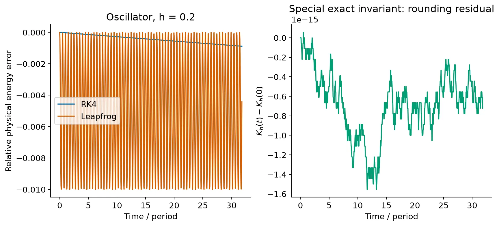
RK4 oscillator energy decays while leapfrog physical energy oscillates and its discrete quadratic invariant remains constant within rounding. — Figure 2:The oscillator at a fixed stable step separates physical energy from the leapfrog invariant $K_h$ . RK4 damps this example; leapfrog preserves $K_h$ up to floating-point effects. Both methods still accumulate phase error.

Higher-Order Symplectic Methods¶

Yoshida’s Fourth-Order Method¶

By composing leapfrog steps with carefully chosen timesteps, we can achieve higher-order accuracy while maintaining symplecticity. The coefficients come from solving order conditions to eliminate $O(h^3)$ errors.

The strange values involving $2^{1/3}$ arise from the algebraic constraints of maintaining symplecticity while achieving fourth-order accuracy:

w_0 = -\frac{2^{1/3}}{2 - 2^{1/3}}, \quad w_1 = \frac{1}{2 - 2^{1/3}}

(16)

Let $S_h$ denote one whole second-order leapfrog step. Apply three steps, in order, with lengths $w_1h$ , $w_0h$ , and $w_1h$ :

S_h^{[4]}=S_{w_1h}\circ S_{w_0h}\circ S_{w_1h}.

(17)

The coefficients satisfy $2w_1+w_0=1$ (advance by total time $h$ ) and $2w_1^3+w_0^3=0$ (cancel the leading symmetric composition error). The middle substep is negative; this is appropriate only when the component flows are defined for those signed substeps.

If we expand kick–drift–kick steps and merge adjacent kicks, the four kick coefficients are $w_1/2,(w_1+w_0)/2,(w_0+w_1)/2,w_1/2$ , while the three drift coefficients are $w_1,w_0,w_1$ . The four kick coefficients are not four whole-leapfrog-step lengths. Confusing these two levels loses fourth order.

Forest–Ruth and symmetric compositions¶

Forest–Ruth and Yoshida constructions belong to this family of fourth-order symmetric splitting methods. When comparing implementations, specify the actual kick/drift sequence: names alone do not identify the update ordering.

Compare diagnostics before choosing a method¶

Use the shared oscillator experiment to compare finite-time position, energy, and phase. A small bounded energy oscillation does not prove a small phase error, and higher order does not remove a method’s step-size restrictions. For an actual Kepler orbit, repeat the comparison at the required eccentricity and duration; the oscillator is a controlled benchmark, not evidence for a thousand-year Earth integration.

When to Use Symplectic Methods¶

Problem Type	Requirement	Candidate method	What to verify
Conservative orbital model	Long-time dynamics	Suitable symplectic splitting	Encounters, step restriction, phase, and energy error
Satellite trajectory	Finite-time position accuracy	Adaptive RK	Position error over the requested duration and force-model adequacy
Collisionless galaxy model	Phase-space dynamics	Symplectic method for a compatible Hamiltonian	Force approximation, resolution, and conserved quantities
Conservative molecular dynamics	Statistical and dynamical observables	Verlet or another appropriate splitting	Fast modes, step size, and sampling of the intended observables
Dissipative system	Correct loss or relaxation	RK for non-stiff problems; implicit method when stiff	Physical decay and time-integration accuracy

Simple Example: Pendulum Dynamics¶

Let’s see symplectic integration in action with a nonlinear pendulum:

import numpy as np

def pendulum_leapfrog(theta0, omega0, g, L, h, n_steps):
    """
    Integrate pendulum with leapfrog
    Second-order fixed-step method; monitor energy error under refinement
    """
    theta, omega = theta0, omega0
    energies = []
    
    for _ in range(n_steps):
        # Initial energy
        E = 0.5*L**2*omega**2 - g*L*np.cos(theta)
        energies.append(E)
        
        # Leapfrog update
        omega_half = omega - 0.5*h*(g/L)*np.sin(theta)
        theta_new = theta + h*omega_half
        omega_new = omega_half - 0.5*h*(g/L)*np.sin(theta_new)
        
        theta, omega = theta_new, omega_new
    
    return energies

For a resolved fixed step, this experiment can show near-conservation beyond the small-angle limit. Repeat it with half the step and monitor the trajectory as well as energy, especially near the separatrix. Large steps need not preserve this behavior.

Answers and reasoning

Each exact-arithmetic kick and drift is symplectic, but their composition follows a discrete approximation to the physical flow. Preserving the two-form does not imply preserving the original Hamiltonian value.
Compare the actual observable, duration, resolution, and cost. RK4 may have smaller short-time state error; resolved leapfrog can have more favorable long-time energy behavior while still accumulating phase error.
Reversing the signed step reverses the symmetric kick–drift–kick sequence. A nonsymmetric symplectic Euler composition is a counterexample to universal reversibility.
The formal modified Hamiltonian differs by $O(h^2)$ for leapfrog; its truncations describe nearby dynamics under appropriate assumptions. The oscillator’s exact quadratic invariant is a special solvable example.
A predetermined sequence of state-independent step lengths composes symplectic maps, but does not supply the same fixed-step energy analysis. Ordinary state-dependent selection generally loses symplecticity. Specialized adaptive constructions require additional variables or a separate formulation.
The two constraints $2w_1+w_0=1$ and $2w_1^3+w_0^3=0$ cancel the cubic composition defect. Solving them introduces the cube root; the coefficients are signed whole-step lengths.

Bridge to Part 4: Stability Analysis¶

You’ve seen the profound difference between local accuracy and geometric preservation. Symplectic methods impose a geometric constraint as well as an accuracy order. Their favorable long-time energy behavior has conditions, and accurate trajectories require enough resolution.

But choosing the right integrator is only part of the challenge. We also need to understand when methods become unstable, how to diagnose problems, and what limits our timestep choices. In Part 4, we’ll analyze stability regions to predict when methods explode and understand the special challenges of stiff equations.

Next: Part 4 - Stability Analysis