The Stellar Blueprint

By the end of this reading, you will be able to:

• State

  the four stellar structure equations and identify the physical principle behind each one

• Explain

  why stellar structure is a coupled ODE problem rather than a single algebra problem

• Derive

  the leading-order toy scaling $L \propto M^3/\kappa$ from the structure equations

• Derive

  a toy mass-radius relation for pp-chain, radiative main-sequence stars

• Derive

  the nuclear-lifetime scaling $\tau_{\rm nuc} \propto M/L$ and explain why massive stars live shorter lives

• State

  the Schwarzschild criterion and explain physically when convection begins

• Distinguish

  fully convective, solar-like, and convective-core main-sequence interiors

• Connect

  the observed main sequence to the underlying stellar-structure physics

Guiding question: why is the mass-luminosity relation so steep — and why do the same four equations set a star’s luminosity, radius, temperature, and lifetime all at once?

For main-sequence stars of similar composition, observations suggest that mass is the dominant control parameter. But that statement is only scientifically useful if we can build a model that explains why changing the mass changes luminosity, radius, temperature, and interior structure so dramatically. In this reading, we assemble the stellar structure equations, show why they must be solved as a coupled system, and then use carefully stated scaling arguments to derive the leading-order physics behind the main sequence. The goal is not to memorize four equations. The goal is to understand why the observed mass-luminosity relation is so steep, why more massive stars are larger and hotter, and why different stars transport energy in different ways.

Concept Throughline

In Module 2, you measured the empirical trend that more massive main-sequence stars are much more luminous. In Readings 1–4, you built the ingredients needed to explain that trend: gravity sets the pressure scale, hydrostatic equilibrium sets the force balance, fusion sets the energy source, and radiation transport sets how hard it is for energy to escape. This reading puts those ingredients together.

The logic chain is:

1. stars are described by radial profiles, so we need differential equations,
2. four coupled structure equations determine how mass, pressure, temperature, and luminosity vary with radius,
3. order-of-magnitude versions of those equations reveal the main-sequence scaling relations,
4. radiative transport can fail when the required temperature gradient becomes too steep,
5. the resulting interior structures explain why different kinds of main-sequence stars look and evolve differently.

The main sequence is not just an observational pattern. It is a structural consequence of stellar physics.

Part 1: The Problem We Are Trying to Explain

Astronomers do not begin this topic from theory alone. We begin from an observable pattern:

• main-sequence stars occupy a narrow band in the HR diagram,
• more massive main-sequence stars are much more luminous,
• the empirical mass-luminosity relation is steep, roughly $L \propto M^{3}$ to $M^{3.5}$ over much of the main sequence.

That is the observable we want to explain. The rest of the reading builds the model and then asks what we can infer from it.

The surprising part is not just that more massive stars are brighter. It is that luminosity increases much faster than mass — that is what we need to explain.

A factor-of-two increase in mass produces roughly an eightfold increase in luminosity. That is not a small effect — it is a structural change. Before reading further, ask yourself: do you expect gravity, temperature, or energy transport to be responsible for this steepness?

Why should a factor-of-two increase in mass produce an increase of roughly one order of magnitude in luminosity? Why are massive stars not just a little brighter, but dramatically brighter? To answer that, we need a theory of stellar interiors.

Part 2: Why Stellar Structure Requires Differential Equations

A star is not described by a single temperature or a single pressure. Those quantities vary continuously from center to surface:

$$M(r), \qquad P(r), \qquad T(r), \qquad L(r), \qquad \rho(r).$$

That means stellar structure is a profile problem. We are not asking for one number. We are asking how each quantity changes with radius. That is why ordinary algebra is not enough. We need a dynamical profile model: a set of differential equations that describes how stellar properties vary with radius.

Why ODEs?

If you want to know the structure of a star, you are really asking: how does each quantity change as you move outward? That is a question about rates of change — and rates of change are what derivatives describe. If a quantity changes continuously with radius, then the natural question is not “what is its value?” but “how fast is it changing?” That is what a derivative tells us.

The stellar structure equations therefore relate how enclosed mass grows with radius, how pressure changes with radius, how temperature changes with radius, and how luminosity changes with radius. Each equation gives one radial rate of change.

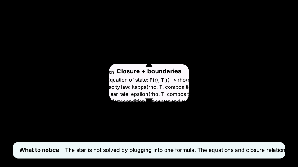
The important point is that the structure equations are not independent recipes. Each equation needs quantities that are determined by the others, so the solution must be self-consistent. A star is not defined by numbers — it is defined by a solution.

Part 3: The Four Equations — The Stellar Blueprint

We now write the four stellar structure equations in their standard spherical form.

Stellar structure equations

The four coupled differential equations — mass conservation, hydrostatic equilibrium, energy generation, and radiative (or convective) transport — that determine how mass, pressure, luminosity, and temperature vary with radius inside a star. Closed by the equation of state, opacity law, and nuclear rate, they are solved as one self-consistent system, not four standalone formulas.

Equation 1: Mass conservation

$$\frac{dM}{dr} = 4\pi r^2 \rho(r)$$

Here $M(r)$ is the mass enclosed inside radius $r$ and $\rho(r)$ is the local density. This equation is geometry. A thin shell of radius $r$ and thickness $dr$ has volume $dV = 4\pi r^2\,dr$, so its mass is $dM = \rho\,dV = 4\pi r^2 \rho\,dr$. Divide by $dr$ and you get the differential form above.

Equation 2: Hydrostatic equilibrium

$$\frac{dP}{dr} = -\frac{G M(r)\rho(r)}{r^2}$$

Here $P(r)$ is the pressure and $G$ is Newton’s gravitational constant. This is force balance: the pressure must decrease outward so that the pressure gradient can support the weight of the overlying gas against gravity.

Equation 3: Energy generation

$$\frac{dL}{dr} = 4\pi r^2 \rho(r)\,\epsilon(r)$$

Here $L(r)$ is the luminosity passing through radius $r$, and $\epsilon(r)$ is the nuclear energy generation rate per unit mass, with units $\mathrm{erg\ g^{-1}\ s^{-1}}$. This is energy conservation inside the star: as you move outward through a shell, the luminosity increases by the energy produced in that shell.

Equation 4: Radiative transport

From Reading 4, the radiative-diffusion luminosity comes from the flux

$$F_{\rm rad} = -\frac{4acT^3}{3\kappa\rho}\frac{dT}{dr},$$

where $a$ is the radiation constant, $c$ is the speed of light, and $\kappa$ is the opacity. Since luminosity is flux times area, $L(r) = 4\pi r^2 F_{\rm rad}$, the radiative temperature gradient can be written as

$$\left(\frac{dT}{dr}\right)_{\rm rad} = -\frac{3\kappa\rho L(r)}{16\pi a c\,r^2 T^3}.$$

Using $a = 4\sigma/c$, this is equivalently

$$\left(\frac{dT}{dr}\right)_{\rm rad} = -\frac{3\kappa\rho L(r)}{64\pi \sigma r^2 T^3}.$$

This equation tells you how steep the temperature gradient must be if radiation alone carries the luminosity.

At this point, you might think: “I have four equations — I can just use them.” But each equation contains quantities defined by the others. That means none of them can be solved independently. This is not four problems. This is one coupled problem. Do not try to memorize these equations; focus on what each one controls in the star.

Equation of state

The thermodynamic relation linking pressure, density, and temperature for stellar material. For an ideal gas it is $P = \rho k_B T/(\mu m_H)$, where $\mu$ is the mean molecular weight. It is one of the closure relations that turns the four structure ODEs into a solvable system.

Quick check

Look back at the four equations and the closure relations. Which equation needs information supplied by another equation? Give at least two examples. Do not answer with “all of them” unless you can explain specifically how.

Part 4: Deriving the Main-Sequence Scalings

We will not solve the full ODE system exactly. Instead, we will build a controlled toy model that extracts the leading-order physics by replacing full radial profiles and local gradients with characteristic scales. This is not the exact stellar solution. It is a deliberately simplified model designed to answer one question: why is the mass-luminosity relation steep at all?

Step 1: Mass conservation gives the density scale

From $dM/dr = 4\pi r^2 \rho$, replace the derivative by a characteristic ratio, $M/R \sim R^2 \rho$. Therefore

$$\rho \sim \frac{M}{R^3}.$$

This is the mean-density scaling: mass divided by volume.

Step 2: Hydrostatic equilibrium gives the pressure scale

Start from $dP/dr = -GM\rho/r^2$ and replace the derivative by a characteristic ratio, $P_c/R \sim GM\rho/R^2$. Insert the density scaling from Step 1:

$$\frac{P_c}{R} \sim \frac{GM}{R^2}\frac{M}{R^3} = \frac{GM^2}{R^5}.$$

Multiply by $R$ to get the hydrostatic pressure scale.

This is the pressure the core must build to hold up the overlying weight. It is an order-of-magnitude scaling, not an exact equality — numerical factors of order unity are dropped, but the dimensional dependence $P_c \propto M^2 R^{-4}$ is physically meaningful.

Step 3: The ideal gas law gives the temperature scale

Use the ideal-gas equation of state, $P \sim \rho k_B T/(\mu m_H)$. At the core scale, $P_c \sim \rho k_B T_c/(\mu m_H)$. Substitute the results from Steps 1 and 2:

$$\frac{GM^2}{R^4} \sim \frac{M}{R^3}\frac{k_B T_c}{\mu m_H}.$$

Cancel one factor of $M$ and simplify to $GM/R \sim k_B T_c/(\mu m_H)$.

The key takeaway is $T_c \propto M/R$. More massive stars tend to have hotter cores, but the radius also matters — so we should not assign a single temperature-mass exponent until we know how $R$ depends on $M$.

Up to this point, we have not used anything about energy transport or nuclear physics. This is purely gravity, pressure support, and the equation of state. That is why the temperature scale emerges from the structure alone.

Step 4: Radiative transport gives a transport-limited luminosity scaling

This step is the heart of the derivation. This is where the steepness enters. Start from the radiative flux form, $F_{\mathrm{rad}} = -(4acT^3/3\kappa\rho)\,dT/dr$. For a scaling argument, replace the gradient by a characteristic ratio, $|dT/dr| \sim T_c/R$. So the characteristic radiative flux is

$$F_{\mathrm{rad}} \sim \frac{4acT_c^3}{3\kappa\rho}\,\frac{T_c}{R} \sim \frac{T_c^4}{\kappa \rho R},$$

where the constants have been dropped because we only want the scaling. Now convert flux to luminosity, $L \sim 4\pi R^2 F_{\mathrm{rad}}$, so that

$$L \sim \frac{R T_c^4}{\kappa \rho}.$$

Substitute the density scaling $\rho \sim M/R^3$ from Step 1:

$$L \sim \frac{R T_c^4}{\kappa (M/R^3)} = \frac{T_c^4 R^4}{\kappa M}.$$

Now substitute the temperature scaling $T_c \propto M/R$ from Step 3:

$$L \sim \frac{(M/R)^4 R^4}{\kappa M} = \frac{M^4}{\kappa M} = \frac{M^3}{\kappa}.$$

This is the clean transport-limited toy luminosity scaling.

At this stage, we have not yet shown that the star actually produces exactly this luminosity. We have shown the luminosity that radiative diffusion can carry for the assumed characteristic structure.

Pause here. Notice what just happened: the radius has dropped out of the scaling entirely. That does not mean radius is irrelevant to stellar structure. It means that under these specific toy assumptions, the leading-order radiative luminosity scaling can be expressed without an explicit radius dependence.

That means luminosity is no longer controlled primarily by size. It is controlled primarily by mass. That is the key reason luminosity depends so steeply on mass — gravity, pressure, temperature, and transport combine in a way that leaves mass as the dominant control parameter. This result depends on the assumptions above, especially that radiative transport sets the temperature gradient and that opacity varies slowly. If those assumptions change, the exponent will change, but the logic linking mass to luminosity remains.

If $\kappa$ is approximately constant, then $L \propto M^3$. That is already close to the observed steep main-sequence relation.

Problem

Hold $M$, $R$, and the characteristic core temperature fixed.

1. If the opacity $\kappa$ doubles, does the transport-limited luminosity increase or decrease?
2. By what factor does it change in the toy scaling?
3. What is the physical reason for that direction?

Write your prediction before doing any algebra.

Why the real exponent is often steeper

The toy result $L \propto M^3$ for similar opacity is not the final word. Real stars do not all have constant opacity, and they do not all burn hydrogen with the same temperature sensitivity. As the opacity law and nuclear physics change across the main sequence, the exponent shifts. Over much of the observed main sequence, the empirical relation is closer to $L \propto M^{3.5}$ than to $M^3$.

That is a success, not a failure of the model. The toy derivation is doing the correct scientific job: it explains why the relation is steep, even though the exact exponent requires more realistic microphysics.

Step 5: A toy mass-radius relation

To get a radius scaling, we now impose a new physical requirement: in a long-lived main-sequence star, energy production in the core must match energy transport out of the star. A crude scaling for the luminosity generated in the core is $L \sim R^3 \rho \epsilon$. For pp-chain hydrogen burning, use the toy scaling $\epsilon \propto \rho T^4$ — that steep temperature dependence is the Gamow-window physics of Reading 3, where a small rise in temperature pushes many more colliding protons into the narrow tunneling window. Then

$$L \sim R^3 \rho (\rho T_c^4) = R^3 \rho^2 T_c^4.$$

Now substitute the density and temperature scalings $\rho \sim M/R^3$ and $T_c \sim M/R$:

$$L \sim R^3 \left(\frac{M}{R^3}\right)^2 \left(\frac{M}{R}\right)^4.$$

Work through the powers carefully:

$$L \sim R^3 \frac{M^2}{R^6} \frac{M^4}{R^4} = \frac{M^6}{R^7}.$$

But from Step 4, the toy transport scaling gave $L \propto M^3/\kappa$.

Set the two luminosity scalings equal:

$$\frac{M^6}{R^7} \propto \frac{M^3}{\kappa} \quad\Longrightarrow\quad R^7 \propto \kappa M^3.$$

For stars of similar opacity, treat $\kappa$ as approximately constant. Then $R^7 \propto M^3$, which gives the toy mass-radius relation

$$R \propto M^{3/7} \approx M^{0.43}.$$

This is shallower than the observed main-sequence radius trend, which is often closer to $R \propto M^{0.6}$ to $M^{0.8}$ over much of the main sequence. That is expected. The toy model uses simplified opacity and energy-generation laws and ignores structural changes across the sequence. Still, it gets the crucial qualitative point right: more massive stars are larger, but luminosity rises more steeply than radius.

That inference depends on the toy assumptions above, especially radiative transport dominance, similar composition, and the simplified pp-chain scaling. A more realistic model changes the exponent, but not the basic logic that mass drives both structure and transport demands.

Step 6: The nuclear lifetime scaling

The nuclear lifetime is approximately the available nuclear fuel divided by the luminosity, where luminosity acts as a proxy for the rate at which the star is spending its usable energy supply. For stars of similar composition, the available fuel scales roughly with mass ($\text{fuel} \propto M$), and the burn rate is the luminosity ($\text{burn rate} \propto L$).

For this leading-order comparison, the prefactors cancel between similar stars, so the scaling reduces to $\tau_{\rm nuc} \propto M/L$.

Using the toy luminosity scaling $L \propto M^3$, we get

$$\tau_{\rm nuc} \propto \frac{M}{M^3} = M^{-2}.$$

Using the more empirical scaling $L \propto M^{3.5}$, we get $\tau_{\rm nuc} \propto M^{-2.5}$. That is why massive stars live much shorter lives. They do have more fuel, but the burn rate rises much faster than the fuel supply. More mass means more fuel, but luminosity grows even faster. That is why massive stars die young.

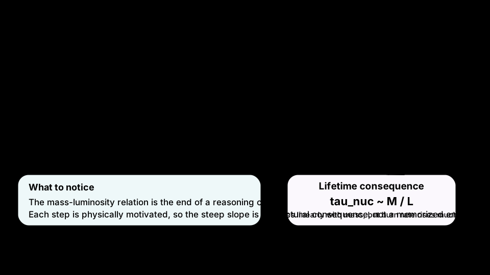
The mass-luminosity relation is not an isolated empirical fact. It is the end of a chain of physical reasoning.

Problem

Use the toy scaling $L \propto M^3$ for stars of similar opacity.

1. Predict qualitatively: if mass doubles, does luminosity increase linearly, quadratically, or more steeply?
2. Now compute the luminosity ratio explicitly.
3. Use $\tau_{\rm nuc} \propto M/L$ to predict the lifetime ratio.
4. Explain in one sentence why the lifetime decreases even though the star has more fuel.

Putting numbers on the blueprint

A scaling is only worth trusting if it survives contact with real stars. So far Module 3 has stayed in exponents; now anchor the chain at the Sun and let it predict.

Worked Example 1The Sun's core temperature, straight from the blueprint

Problem

Recover the Sun’s central temperature from the structure scaling $T_c \sim \mu G M_\odot m_p/(k_B R_\odot)$ alone, with $\mu = 0.6$, $G = 6.674\times10^{-8}$, $M_\odot = 2.0\times10^{33}\,\mathrm{g}$, $m_p = 1.67\times10^{-24}\,\mathrm{g}$, $k_B = 1.38\times10^{-16}\,\mathrm{erg\,K^{-1}}$, $R_\odot = 7.0\times10^{10}\,\mathrm{cm}$.

Step·Numerator

$(0.6)(6.674\times10^{-8})(2.0\times10^{33})(1.67\times10^{-24}) \approx 1.34\times10^{2}$.

Step·Denominator

$(1.38\times10^{-16})(7.0\times10^{10}) \approx 9.66\times10^{-6}$.

Dimensional check

$\dfrac{(\mathrm{cm^3\,g^{-1}\,s^{-2}})(\mathrm{g})(\mathrm{g})}{(\mathrm{erg\,K^{-1}})(\mathrm{cm})} = \mathrm{K}$, since $1\,\mathrm{erg} = 1\,\mathrm{g\,cm^2\,s^{-2}}$. ✓

Result

$T_c \approx (1.34\times10^2)/(9.66\times10^{-6}) \approx 1.4\times10^{7}\,\mathrm{K} = 14\,\mathrm{MK}$. The measured solar core is $15\,\mathrm{MK}$ — gravity, force balance, and the gas law alone land within $10\%$, no nuclear physics required.

The main sequence, predicted. Anchor the toy scalings at the Sun ($L_\odot$, $R_\odot$, $T_c = 15\,\mathrm{MK}$, $\tau_\odot \approx 10\,\mathrm{Gyr}$) and read off the rest of the sequence:

Three lessons fall straight out of the numbers. (1) Core temperature barely moves — a factor of $\sim 5$ across a factor of $20$ in mass — because $T_c \propto M^{4/7}$ is weak. (2) The lifetime swings by a factor of $\sim 400$: massive stars die young because they are profligate, not because they are fuel-starved. (3) The toy $M^3$ overpredicts $L$ at low mass and underpredicts it at high mass — the true exponent is nearer $3.5$, which is the audit’s next line item.

Numeric answer

Use the toy scaling $L \propto M^3$, anchored at the Sun, to predict the luminosity of a $4\,M_\odot$ main-sequence star, in units of $L_\odot$.

Your answer

One number the toy gets wrong — on purpose. Push the absolute prefactor through, $L \sim (16\pi a c/3\kappa)(\mu G m_p/k_B)^4 M^3$, and the Sun’s luminosity comes out roughly $10^3\times$ too high. The exponent is right; the coefficient is badly off — and the culprit is a single assumption, $T(r)\to T_c$ everywhere. Real stars are far cooler than $T_c$ across most of their volume, and $L\propto T^4$ punishes that error enormously. That is the one-zone row of the audit — and exactly what the next section stacks up and stress-tests.

Part 5: When Radiation Fails — Convection

The radiative-transport equation does more than tell us how energy flows. It also tells us when radiation is no longer able to carry the required luminosity stably by itself. When that happens, convection can begin.

The physical idea

Imagine a small blob of gas displaced upward inside a star. As it rises, the pressure around it drops. The blob expands and cools. Now compare two temperature gradients:

• the adiabatic gradient: how fast the blob cools as it expands without exchanging heat,
• the radiative gradient: how fast the background star’s temperature would drop if radiation alone carried the luminosity.

Adiabatic gradient

The temperature gradient $\nabla_{\rm ad} = (d\ln T/d\ln P)_{\rm ad}$ a gas parcel follows as it rises and expands without exchanging heat with its surroundings. It sets the cooling rate of a displaced parcel and is the stability reference in the Schwarzschild criterion.

Radiative gradient

The temperature gradient $\nabla_{\rm rad} = (d\ln T/d\ln P)_{\rm rad}$ the background star would need if radiative diffusion alone carried the local luminosity. It steepens with high opacity, high density, high luminosity, low temperature, or small radius — and when it exceeds the adiabatic gradient, convection sets in.

If the surroundings cool more rapidly than the blob does, then the blob remains warmer and less dense than its environment. It stays buoyant and continues to rise. That is convective instability.

Convective instability

The condition under which a displaced gas parcel keeps rising instead of returning: when the radiative gradient is steeper than the adiabatic gradient, the surroundings cool faster than the parcel, so it stays buoyant. It is the onset criterion for convection, captured formally by the Schwarzschild criterion.

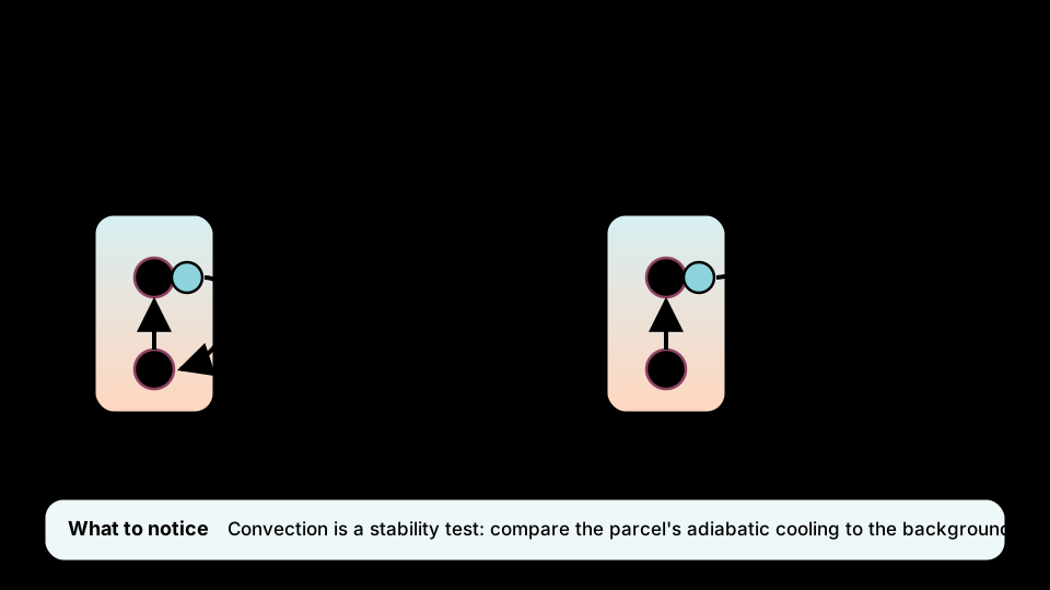
This is why convection is a stability problem, not just the slogan “hot gas rises.” What matters is the comparison between the parcel’s adiabatic cooling and the background radiative gradient. The question is not “is the gas hot?” The question is “does the environment cool faster than the parcel?”

The Schwarzschild criterion

The standard criterion is written in logarithmic form using the Schwarzschild criterion:

$$\nabla_{\rm rad} > \nabla_{\rm ad}, \qquad \nabla \equiv \frac{d\ln T}{d\ln P}.$$

Schwarzschild criterion

The condition for convective instability in a chemically homogeneous layer: convection occurs where the radiative gradient exceeds the adiabatic gradient, $\nabla_{\rm rad} > \nabla_{\rm ad}$, with $\nabla \equiv d\ln T/d\ln P$. Below threshold the layer stays radiative; above it, a displaced parcel remains buoyant and convection carries the energy.

At the level of physical intuition, this means the radiative temperature drop is too steep for stability, so a displaced parcel remains buoyant instead of returning to its original position. In words:

• if radiation can carry the luminosity with a gentle enough gradient, the region stays radiative,
• if radiation would require too steep a gradient, convection begins.

Why compare gradients per unit pressure instead of per unit radius? A displaced parcel matches the pressure of its new surroundings almost instantly — pressure equilibrates at the sound-crossing time, long before heat can leak across the parcel. At a fixed depth the parcel and the background therefore sit at the same $P$, so recasting the gradient in the dimensionless form $\nabla \equiv d\ln T/d\ln P$ divides out the hydrostatic structure $dP/dr$ they share and isolates the one thing that decides stability: how the parcel’s temperature responds to pressure compared with the background’s.

What makes the radiative gradient steep?

From the radiative-transport equation, that same radiative gradient — written here in its un-normalized $|dT/dr|$ form — scales as

$$\left|\frac{dT}{dr}\right|_{\rm rad} \propto \frac{\kappa \rho L}{T^3 r^2}.$$

So the radiative gradient becomes steeper when opacity $\kappa$ is high, density $\rho$ is high, luminosity $L$ is high, temperature $T$ is low, or radius $r$ is small. That already suggests two places where convection might appear:

1. cool, opaque outer layers, where radiation struggles to get through,
2. very luminous cores, where too much energy must pass through a small area.

Three main-sequence interior regimes

1. Very low-mass stars: often fully convective

At the lowest main-sequence masses, the combination of cool temperatures, high opacity, and structural properties can make convection efficient throughout most or all of the star. Result: many stars below roughly $M \lesssim 0.35\,M_\odot$ are close to fully convective.

2. Solar-like stars: radiative cores and convective envelopes

For stars like the Sun, the core is hot and fully ionized, so the opacity is relatively low and radiation can carry the energy without requiring an unstable gradient. But the outer envelope is cooler and more opaque. There, radiative transport becomes inefficient and convection takes over. Result: stars of roughly solar mass typically have radiative cores and convective envelopes.

3. Higher-mass stars: convective cores and radiative envelopes

In more massive stars, the core temperature becomes high enough that the CNO cycle dominates hydrogen burning. The CNO cycle is much more temperature-sensitive than the pp chain, so energy generation becomes strongly concentrated toward the center. That concentrates a large luminosity into a small inner region, making the required radiative gradient very steep. The core becomes convective. Meanwhile, the envelope is hot and relatively transparent, so radiation can often carry the energy there. Result: stars above roughly $M \gtrsim 1.3$ to $1.5\,M_\odot$ typically have convective cores and radiative envelopes.

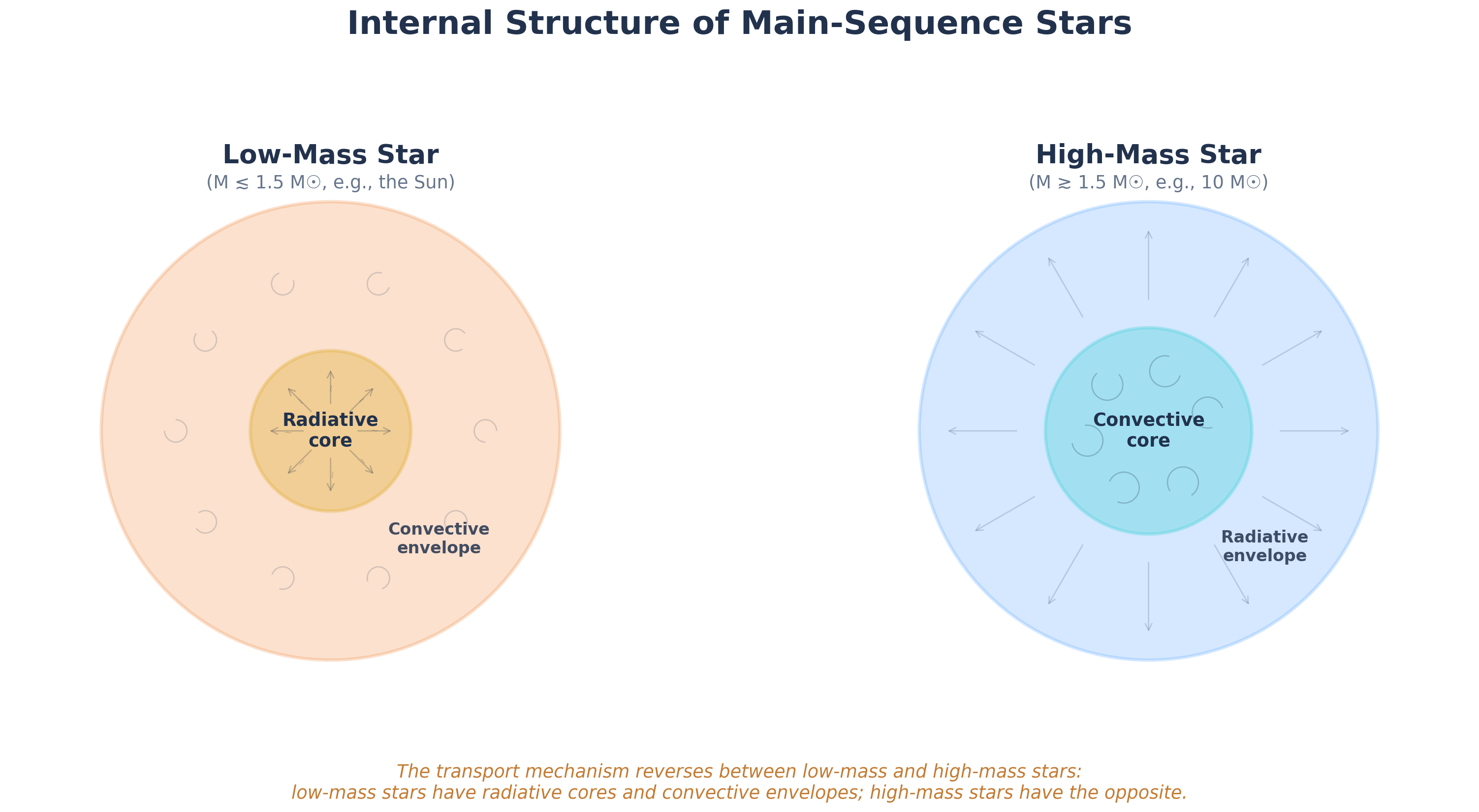
This schematic compares the solar-like and high-mass archetypes. The very lowest-mass main-sequence stars are a third regime: many are nearly fully convective and are therefore not represented by the Sun-like panel.

Multiple choice

Using $|dT/dr|_{\rm rad} \propto \kappa \rho L/(T^3 r^2)$, which change in an outer envelope is more likely to trigger convection?

Increasing the opacity — it steepens the radiative gradientDecreasing the opacity

Part 6: The Main Sequence Explained

We can now connect the whole argument.

Why stars spend most of their lives there

Main-sequence stars are in long-lived thermal balance: fusion in the core generates energy, that energy is transported to the surface, and the luminosity leaving the surface matches the energy production rate on long timescales. This balance is stable because hydrogen-burning stars have a self-regulating thermal feedback:

• if the core produces too much energy, the star expands, expansion lowers the core temperature, and fusion weakens,
• if the core produces too little energy, the star contracts, contraction raises the core temperature, and fusion strengthens.

That self-regulation is why hydrogen burning can last for billions of years.

Pressure-test the model

Every scaling in Module 3 was bought with an assumption, and we have kept the receipts reading by reading. Here is the full assumption audit, stacked, with the place each line finally fails:

Read the last two columns and the pattern is unmistakable. What is robust is the steep exponent near 3; what shifts — to $3.5$, or for the most massive radiation-dominated stars back toward $1$ — is set by exactly which audited assumption gives way. The coefficient was never the point. This is Kelvin’s lesson from Reading 1, paid forward across the entire module: the arithmetic is honest, the model is approximate, and the audit tells you precisely where to look when a real star disagrees. Naming the assumption is not a disclaimer — it is the most useful output of the whole derivation.

Reference Tables

The four stellar structure equations

Closure relations

Main-sequence scaling relations

Interior regimes across the main sequence

Retrieval — equation: luminosity-mass-scaling▸

Summary: From Equations to the HR Diagram

The most important ideas from this reading are:

• Stars require differential equations because they are described by radial profiles, not single numbers.
• The four stellar structure equations govern mass, pressure, temperature, and luminosity as functions of radius.
• Those equations must be combined with closure relations such as the equation of state, opacity law, and nuclear energy generation law.
• A toy scaling analysis gives $L \propto M^3/\kappa$, which explains why the main-sequence mass-luminosity relation is so steep.
• A toy pp-chain, radiative model gives $R \propto M^{3/7}$, which captures the qualitative trend that more massive stars are larger.
• The nuclear lifetime scales as $\tau_{\rm nuc} \propto M/L$, so massive stars live much shorter lives because luminosity rises more steeply than fuel supply.
• Convection appears when radiative transport would require too steep a temperature gradient.
• The main sequence is a mass sequence in thermal equilibrium, not just an observational catalog.

Glossary

Adiabatic gradient

The temperature gradient $\nabla_{\rm ad} = (d\ln T/d\ln P)_{\rm ad}$ a gas parcel follows as it rises and expands without exchanging heat with its surroundings. It sets the cooling rate of a displaced parcel and is the stability reference in the Schwarzschild criterion.

Convective instability

The condition under which a displaced gas parcel keeps rising instead of returning: when the radiative gradient is steeper than the adiabatic gradient, the surroundings cool faster than the parcel, so it stays buoyant. It is the onset criterion for convection, captured formally by the Schwarzschild criterion.

Equation of state

The thermodynamic relation linking pressure, density, and temperature for stellar material. For an ideal gas it is $P = \rho k_B T/(\mu m_H)$, where $\mu$ is the mean molecular weight. It is one of the closure relations that turns the four structure ODEs into a solvable system.

Radiative gradient

The temperature gradient $\nabla_{\rm rad} = (d\ln T/d\ln P)_{\rm rad}$ the background star would need if radiative diffusion alone carried the local luminosity. It steepens with high opacity, high density, high luminosity, low temperature, or small radius — and when it exceeds the adiabatic gradient, convection sets in.

Schwarzschild criterion

The condition for convective instability in a chemically homogeneous layer: convection occurs where the radiative gradient exceeds the adiabatic gradient, $\nabla_{\rm rad} > \nabla_{\rm ad}$, with $\nabla \equiv d\ln T/d\ln P$. Below threshold the layer stays radiative; above it, a displaced parcel remains buoyant and convection carries the energy.

Stellar structure equations

The four coupled differential equations — mass conservation, hydrostatic equilibrium, energy generation, and radiative (or convective) transport — that determine how mass, pressure, luminosity, and temperature vary with radius inside a star. Closed by the equation of state, opacity law, and nuclear rate, they are solved as one self-consistent system, not four standalone formulas.