Distance & Parallax

By the end of this reading, you will be able to:

• Define

  angular measure in all its forms (degrees, arcminutes, arcseconds, radians) and convert between them

• Derive

  the small-angle approximation from geometry and explain its physical meaning

• Define

  the parallax angle and the parsec, and the relation $d_{\rm pc} = 1/p_{\rm arcsec}$

• Calculate

  stellar distances from parallax measurements

• Explain

  why distance is the “master key” to measuring all other stellar properties

• Derive

  the inverse-square law geometrically and by dimensional analysis

• Apply

  the flux-luminosity-distance relation to infer luminosity, and name the Observable → Model → Inference steps

Part 1: The Distance Problem — Why It Matters

The Fundamental Challenge

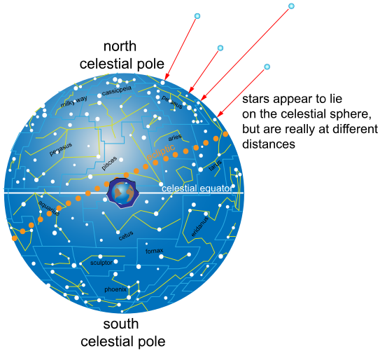
Look up on any clear night. Every star is a point of light — a tiny, seemingly dimensionless dot. This simplicity conceals one of the deepest challenges in astronomy: how far away is it?

Unlike nearby objects on Earth, we cannot pace out a star’s distance or send a probe and measure travel time. We must infer distance from the light alone — and that inference is fraught with ambiguity. A faint, distant star can appear the same brightness as a near, luminous one. Without knowing how far a star is, we cannot determine its true brightness — its intrinsic power output, or luminosity. And without luminosity, we cannot build the Hertzsprung-Russell diagram, the map that reveals stellar properties and evolution.

Hertzsprung-Russell diagram

A plot of stellar luminosity (vertical axis, logarithmic) versus effective temperature (horizontal axis) that reveals stellar properties and evolutionary states. Building it requires knowing luminosity — which requires distance.

This is the starting point for stellar astrophysics: everything that follows — radius, composition, age, fate — depends on first solving the distance puzzle. And it is hard, because stars are points with no measurable angular size, and parallax (the apparent shift as Earth orbits) is tiny: even the nearest star shifts by less than one arcsecond across Earth’s orbital diameter.

The Observable → Model → Inference Framework

This lecture is organized around a single framework that threads through all of astronomy:

• Observable: we measure a star’s position at different times of year (it shifts slightly against the distant background) and its brightness (the flux reaching Earth). Both are directly measurable.
• Model: we build a geometric model of Earth’s orbit and apply the small-angle approximation, and we model the star as a point source radiating isotropically. These are assumptions that connect observations to what we want to know.
• Inference: from the position shift we calculate distance; from flux and distance we calculate luminosity. These are derived — not directly measured.

Models can be wrong and assumptions can fail. Good scientists always ask: what am I assuming, and what would break it? In Parts 2–3 we build the angular toolkit; in Part 4 we apply it to parallax; Part 5 develops the inverse-square law two ways; Part 6 combines them to infer luminosity; Part 7 previews standard candles.

Part 2: Angular Measure — The Language of the Sky

Before we can talk about parallax, we need a language for measuring angles.

Degrees, Arcminutes, and Arcseconds

The full sky is divided into 360 degrees ($^\circ$) — a choice inherited from the Babylonian base-60 system. The Sun and Moon each span about $0.5^\circ$. For stellar parallax we need finer divisions: one degree is 60 arcminutes ($'$), and one arcminute is 60 arcseconds ($''$), so $1'' = 1/3600$ degree. This is the scale of stellar parallax — Proxima Centauri shifts by $0.77''$ as Earth orbits.

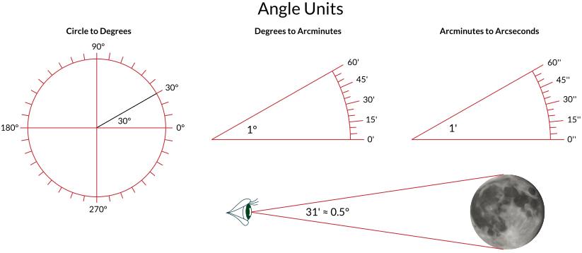
Problem

Convert (a) 1 degree, (b) 5 arcminutes, (c) 0.5 degrees to arcseconds.

Arcsecond

An angular unit equal to $1/3600$ of a degree (or $1/60$ of an arcminute) — the standard unit for stellar parallax. It measures angle, never distance.

Radians — The Natural Unit

Degrees are human convention; physics prefers the radian, which emerges directly from geometry: 1 radian is the angle subtended by an arc whose length equals the circle’s radius.

Radian

The natural (dimensionless) angle unit: the angle subtended by an arc whose length equals the radius, so angle = arc length / radius. A full circle is $2\pi$ rad, and $1\ \text{rad} = 206{,}265''$.

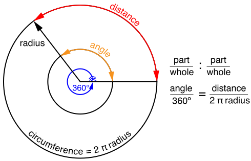
Because it’s a ratio of lengths, a radian is dimensionless: $\text{angle (rad)} = \text{arc length}/\text{radius}$. A full circle is $2\pi$ rad, so $1\ \text{rad} = 360^\circ/2\pi \approx 57.3^\circ$.

The Critical Conversion: Arcseconds to Radians

Stellar parallax is measured in arcseconds, but the small-angle formula produces radians. Converting:

$1\ \text{rad} = \frac{360^\circ}{2\pi} = \frac{360 \times 3600''}{2\pi} = \frac{1{,}296{,}000''}{2\pi} \approx 206{,}265''.$

$\boxed{1\ \text{rad} = 206{,}265'' \qquad 1'' = \frac{1}{206{,}265}\ \text{rad} \approx 4.85 \times 10^{-6}\ \text{rad}}$

Part 3: Geometric Foundations — The Small-Angle Approximation

We need a relationship connecting angular size, true size, and distance.

The Geometric Picture

Consider an observer at distance $d$ from a small object of true size $s$, which subtends an angle $\alpha$. Drawing the triangle, for small angles the arc subtended by the object’s edge is approximately its true size, and the arc’s radius is the distance.

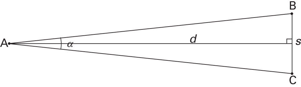
By the definition of angle in radians, $\alpha \approx \text{arc length}/\text{radius} \approx s/d$. This is the small-angle approximation:

Angular size is inversely proportional to distance: a distant object appears small, a nearby one large. The angle $\alpha$ must be in radians for the formula to work without a conversion factor.

Small-angle approximation

For small angles ($\alpha \ll 1$ rad), $\sin\alpha \approx \tan\alpha \approx \alpha$, giving the clean geometric relation $s = \alpha d$ between physical size, angular size, and distance.

Numeric answer

The Moon subtends about $0.5^\circ$; its distance is $\approx 3.84 \times 10^{10}$ cm. Estimate its true diameter.

Your answer

The approximation holds while $\alpha \lesssim 0.1$ rad (roughly 5–6 degrees); beyond that, use the exact trigonometry. In astronomy we rarely exceed a degree, so it’s superb for parallax, galaxy sizes, and telescope resolution.

Part 4: Parallax — Distance from Baseline Geometry

Now we apply the small-angle formula to the most direct distance technique: parallax — use a long baseline and measure the angular shift of a nearby object against fixed background objects.

The Parallax Angle

Hold your finger at arm’s length and blink between eyes: it shifts against the background, and the farther away it is, the smaller the shift. That’s parallax. The geometry is the small-angle formula with the baseline $b$ playing the role of “size,” the parallax angle $p$ playing “angle,” and the distance $d$ what we want. Substituting $b = p\,d$ and solving:

Here $b$ is the baseline, $p$ the parallax angle (radians), and $d$ the distance in the same units as $b$. This works for any baseline and any observer.

The distance you can probe is set by the baseline: your eyes ($b \approx 7$ cm) give depth perception to a few meters; Earth’s orbit ($b = 1$ AU) makes stellar parallax possible; a larger baseline reaches proportionally farther at the same angular precision. The physics is always $d = b/p$ — only the baseline changes.

Stellar Parallax: Earth’s Orbit as Baseline

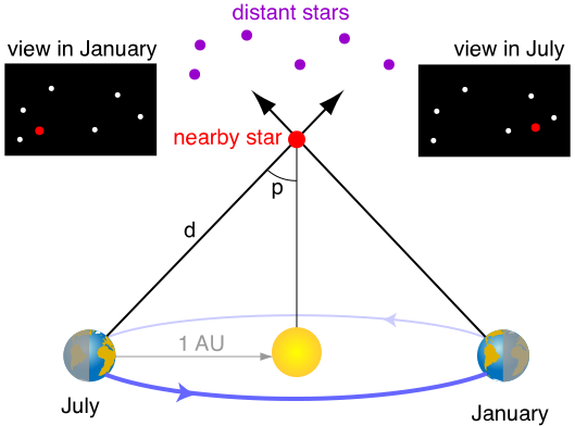
As Earth moves from one side of the Sun to the other, a nearby star shifts against the distant background. We define the parallax angle $p$ as half the total shift — the angle subtended by Earth’s orbital radius (1 AU), not its diameter.

Parallax angle

The apparent angular shift of a nearby star as Earth orbits, defined as half the total six-month shift — the angle Earth’s 1 AU orbital radius subtends as seen from the star. Measured in arcseconds.

From General Parallax to the Parsec

Substituting Earth’s baseline $b = 1$ AU and converting to arcseconds gives $d = 206{,}265\ \text{AU} / p('')$. Astronomers then define a unit to make this clean: one parsec is the distance at which 1 AU subtends $1''$, so $1\ \text{pc} = 206{,}265$ AU. The relation becomes:

A star with $p = 0.5''$ is at 2 pc; $p = 0.1''$ is at 10 pc. The name “parsec” is parallax-arcsecond — it works only because Earth’s 1 AU baseline and the arcsecond are baked into the definition.

Parsec

The distance at which a star shows a parallax of $1''$ (with Earth’s 1 AU baseline): $1\ \text{pc} = 206{,}265\ \text{AU} = 3.09 \times 10^{18}\ \text{cm} = 3.26$ light-years. The natural unit for stellar distances.

For reference: $1\ \text{pc} = 3.09 \times 10^{18}$ cm $= 3.26$ light-years, and $1$ kpc $= 1000$ pc.

Worked Example 1Proxima Centauri

Problem

Proxima Centauri, the nearest known star, has parallax $p = 0.768''$. Find its distance in parsecs and centimeters.

Step·Apply the parsec form

$d = \frac{1}{p} = \frac{1}{0.768''} = 1.30\ \text{pc}$

Step·Convert to CGS

$d = 1.30\ \text{pc} \times 3.09 \times 10^{18}\ \text{cm/pc} = 4.02 \times 10^{18}\ \text{cm}$

Dimensional check

$1/('')$ gives pc by the definition of the parsec; pc $\times$ (cm/pc) leaves cm ✓.

Result

$d \approx 1.30$ pc $\approx 4.0 \times 10^{18}$ cm. Sanity check: nearby stars fall in the 1–5 pc range ✓. Its parallax was barely measurable from the ground — which is why parallax was historically so hard.

Numeric answer

Estimate the parallax angle for a star at 1000 pc.

Your answer

Part 5: The Inverse-Square Law — Two Derivations

The second pillar of distance measurement: how light spreads from a star to Earth.

Predict First

Reason about why before reading the derivation.

If you move twice as far from a light source, by what factor does the brightness change? What about 10 times farther?

The two derivations below confirm your reasoning.

Geometric Derivation: Concentric Spheres

A star of luminosity $L$ (total power radiated in all directions) sits at the center of a sphere. At distance $d$ the energy is spread over area $A = 4\pi d^2$, so the flux (power per unit area) is

$F(d) = \frac{L}{4\pi d^2}.$

The same total energy $L$ flows through every spherical shell; at larger radius the area grows as $d^2$, so the flux drops as $1/d^2$. Double the distance, quarter the flux; ten times farther, one-hundredth. The $4\pi$ is the full solid angle of a sphere.

Dimensional Analysis Derivation

Assume $F \propto L^a d^b$ and match dimensions in $[M\,L\,T]$: flux $[M\,L^0\,T^{-3}]$, luminosity $[M\,L^2\,T^{-3}]$, distance $[L]$.

$[M\,L^0\,T^{-3}] = [M^a\,L^{2a+b}\,T^{-3a}] \;\Rightarrow\; a = 1,\quad 2a + b = 0 \Rightarrow b = -2.$

So $F \propto L/d^2$; the constant $1/(4\pi)$ comes from geometry, which dimensional analysis can’t supply. Two independent routes give the same $1/d^2$ scaling — that’s confidence.

The Flux-Luminosity-Distance Equation

This is the cornerstone of all stellar luminosity measurements. It rearranges three ways: given $L$ and $d$, find flux ($F = L/4\pi d^2$); given $F$ and $d$, find luminosity ($L = 4\pi d^2 F$ — what builds the HR diagram); given $L$ and $F$, find distance ($d = \sqrt{L/4\pi F}$ — standard candles).

Part 6: From Distance to Luminosity

Now we combine parallax and the inverse-square law: measured distance plus measured brightness gives intrinsic luminosity — the real power of stellar astrophysics.

Worked Example 2The Solar Constant and Solar Luminosity

Problem

The flux from the Sun at Earth is $F_\odot = 1.4 \times 10^{6}\ \mathrm{erg\,cm^{-2}\,s^{-1}}$ at $d = 1$ AU $= 1.5 \times 10^{13}$ cm. Find the solar luminosity.

Step·Rearrange and substitute

$L_\odot = 4\pi d^2 F = 4\pi\,(1.5 \times 10^{13}\ \text{cm})^2 (1.4 \times 10^{6}\ \mathrm{erg\,cm^{-2}\,s^{-1}})$

Step·Evaluate

$= 4\pi \times (2.25 \times 10^{26}\ \text{cm}^2)(1.4 \times 10^{6}) \approx 3.96 \times 10^{33}\ \mathrm{erg\,s^{-1}}$

Dimensional check

$\text{cm}^2 \times \mathrm{erg\,cm^{-2}\,s^{-1}} = \mathrm{erg\,s^{-1}}$ — a power ✓.

Result

$L_\odot \approx 3.96 \times 10^{33}\ \mathrm{erg\,s^{-1}}$, within ~4% of the accepted $3.828 \times 10^{33}$. This is how we know the Sun’s luminosity — and every star on the HR diagram was placed by this identical method.

Error Propagation: Why Precision Matters

Predict First

Make a prediction and reason about why before reading on.

If Gaia improves parallax precision by 100x over Hipparcos, does the luminosity uncertainty improve by the same factor, more, or less?

Trace the chain below.

Since $d = 1/p$, fractional uncertainties pass straight through: $\delta d/d = \delta p/p$. But $L = 4\pi d^2 F$ has distance squared, so $\delta L/L \approx 2\,(\delta d/d)$. The chain: 10% parallax uncertainty → ~10% distance → ~20% luminosity. This is why Gaia’s $100\times$ parallax improvement translates to a $100\times$ improvement in luminosity precision.

Problem

A star has $p = 0.1''$ and flux $F = 10^{-11}\ \mathrm{erg\,cm^{-2}\,s^{-1}}$. Find its distance (pc and cm) and luminosity (in $L_\odot$).

Distance Is the Master Key

Every other stellar property ultimately depends on distance:

$\text{Parallax} \xrightarrow{\;d = 1/p\;} \text{Distance} \xrightarrow{\;+\,F\;} \text{Luminosity} \xrightarrow{\;+\,T\;} \text{HR Diagram}$

Distance + brightness gives luminosity (this lecture); luminosity + temperature gives radius (next lecture, via Stefan-Boltzmann); distance + spectrum gives composition; distance + binary radial velocity gives mass. Each link amplifies errors, which is why precision parallax pulls the whole chain taut.

Worked Example 3The Full Measurement Chain

Problem

From Gaia and photometry: $p = 0.214''$, $F = 1.1 \times 10^{-7}\ \mathrm{erg\,cm^{-2}\,s^{-1}}$. What kind of star is this?

Step·Parallax to distance

$d = 1/0.214 = 4.67\ \text{pc} = 1.44 \times 10^{19}\ \text{cm}$

Step·Distance + flux to luminosity

$L = 4\pi d^2 F = 4\pi (1.44\times10^{19})^2 (1.1\times10^{-7}) \approx 2.9 \times 10^{32}\ \mathrm{erg\,s^{-1}}$

Dimensional check

$\text{cm}^2 \times \mathrm{erg\,cm^{-2}\,s^{-1}} = \mathrm{erg\,s^{-1}}$ ✓.

Result

$L/L_\odot \approx 0.075$ — about 13× dimmer than the Sun. At 4.67 pc, a late-K or early-M dwarf: a small, cool red star on the lower main sequence. A tiny angular shift plus a brightness measurement reveals the star’s nature.

Part 7: Standard Candles — A Preview

Parallax reaches ~100 pc from the ground, ~10 kpc with Gaia — too close for most of the Milky Way, let alone other galaxies. Beyond that, we invert the inverse-square law: if we know a source’s intrinsic luminosity, we measure its flux and infer distance, $d = \sqrt{L/(4\pi F)}$. Such objects of known luminosity are standard candles (defined in Lecture 1).

Worked Example 4Standard-Candle Distance

Problem

A Cepheid has known $L = 10{,}000\,L_\odot = 3.8 \times 10^{37}\ \mathrm{erg\,s^{-1}}$ (from its pulsation period) and measured $F = 1.0 \times 10^{-14}\ \mathrm{erg\,cm^{-2}\,s^{-1}}$. Find its distance.

Step·Invert the inverse-square law

$d = \sqrt{\frac{L}{4\pi F}} = \sqrt{\frac{3.8\times10^{37}}{4\pi (1.0\times10^{-14})}} \approx \sqrt{3.0\times10^{50}\ \text{cm}^2} \approx 1.7 \times 10^{25}\ \text{cm}$

Dimensional check

$\sqrt{\mathrm{erg\,s^{-1}} / (\mathrm{erg\,cm^{-2}\,s^{-1}})} = \sqrt{\text{cm}^2} = \text{cm}$ ✓.

Result

$d \approx 1.7 \times 10^{25}$ cm $\approx 5.5$ Mpc — well beyond the Milky Way, in a nearby galaxy, far past parallax reach.

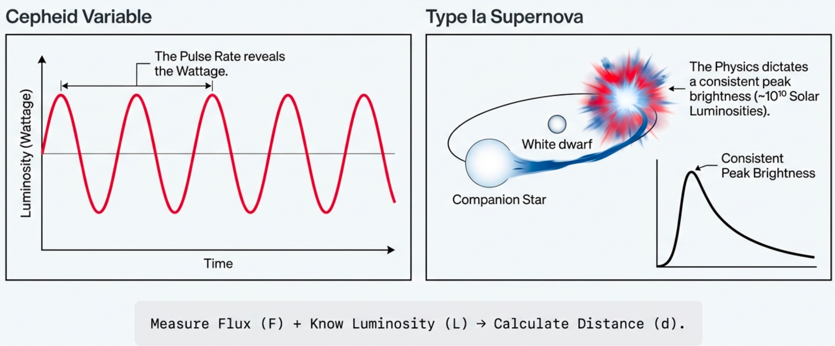
Cepheid variables pulsate over days to months; Henrietta Leavitt (1912) found that pulsation period tracks luminosity, so measuring the period gives $L$. Hubble used Cepheids in Andromeda in the 1920s to prove it is a separate galaxy. Type Ia supernovae — thermonuclear explosions of white dwarfs — reach a consistent peak ($\sim$ a few $\times 10^9\,L_\odot$), making them standard candles to cosmological distances; in 1998 they revealed the accelerating expansion (dark energy, 2011 Nobel Prize).

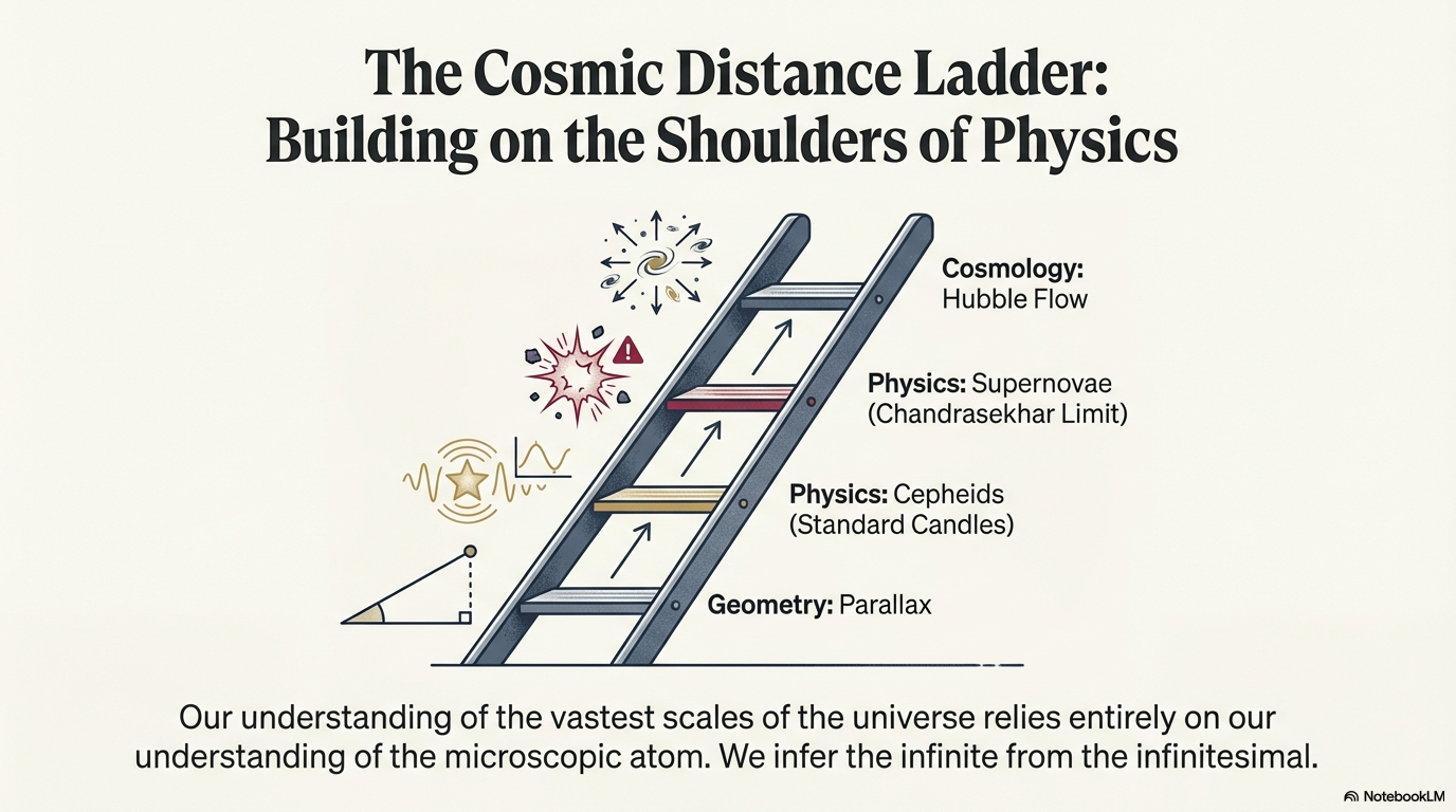
The cosmic distance ladder chains the methods: parallax (geometry) calibrates nearby Cepheids; Cepheids calibrate Type Ia supernovae; each rung rests on the one below. The entire cosmic distance scale ultimately rests on getting nearby parallaxes right — which is why Gaia’s improvement rippled through all of cosmology.

Summary: Observable → Model → Inference

Each step has assumptions: parallax assumes Earth’s orbit is known; the inverse-square law assumes isotropic emission and no absorption; standard candles assume correct calibration. Good science always asks: what could go wrong?

Retrieval — equation: flux-luminosity-distance▸

Looking Ahead

This lecture gave you distance and luminosity — one axis of the HR diagram. Next (Surface Flux & Colors) we apply thermal physics (Stefan-Boltzmann, Wien) to get effective temperature and radius; later lectures add composition (spectra), mass (binary orbits), and the magnitude system, before we assemble the full HR diagram.

Glossary

Arcsecond

An angular unit equal to $1/3600$ of a degree (or $1/60$ of an arcminute) — the standard unit for stellar parallax. It measures angle, never distance.

Hertzsprung-Russell diagram

A plot of stellar luminosity (vertical axis, logarithmic) versus effective temperature (horizontal axis) that reveals stellar properties and evolutionary states. Building it requires knowing luminosity — which requires distance.

Parallax angle

The apparent angular shift of a nearby star as Earth orbits, defined as half the total six-month shift — the angle Earth’s 1 AU orbital radius subtends as seen from the star. Measured in arcseconds.

Parsec

The distance at which a star shows a parallax of $1''$ (with Earth’s 1 AU baseline): $1\ \text{pc} = 206{,}265\ \text{AU} = 3.09 \times 10^{18}\ \text{cm} = 3.26$ light-years. The natural unit for stellar distances.

Radian

The natural (dimensionless) angle unit: the angle subtended by an arc whose length equals the radius, so angle = arc length / radius. A full circle is $2\pi$ rad, and $1\ \text{rad} = 206{,}265''$.

Small-angle approximation

For small angles ($\alpha \ll 1$ rad), $\sin\alpha \approx \tan\alpha \approx \alpha$, giving the clean geometric relation $s = \alpha d$ between physical size, angular size, and distance.