The Boundaries of Stardom

Section 4 of 6

The Maximum Stellar Mass

Part 4: The Maximum Stellar Mass

Hubble Space Telescope image of Eta Carinae showing a brilliant central star surrounded by two large bipolar lobes of ejected gas and dust (the Homunculus Nebula), glowing in orange-white with fainter red nebulosity extending outward. — Figure 1Eta Carinae — one of the most massive and luminous stars in the Milky Way (~100-150 solar masses, ~5e6 solar luminosities). It sits near the Eddington limit, where radiation pressure nearly overwhelms gravity. The bipolar Homunculus Nebula was ejected during the Great Eruption of the 1840s. This is what happens when a star pushes against the maximum-mass ceiling.NASA/ESA/HST; Processing: Judy Schmidt

The Eddington Limit Revisited

In Module 3 (radiation transport), we introduced the Eddington luminosity — the maximum luminosity a star can sustain in hydrostatic equilibrium. The ceiling is Reading the Limit again — a second balance, solved the same way:

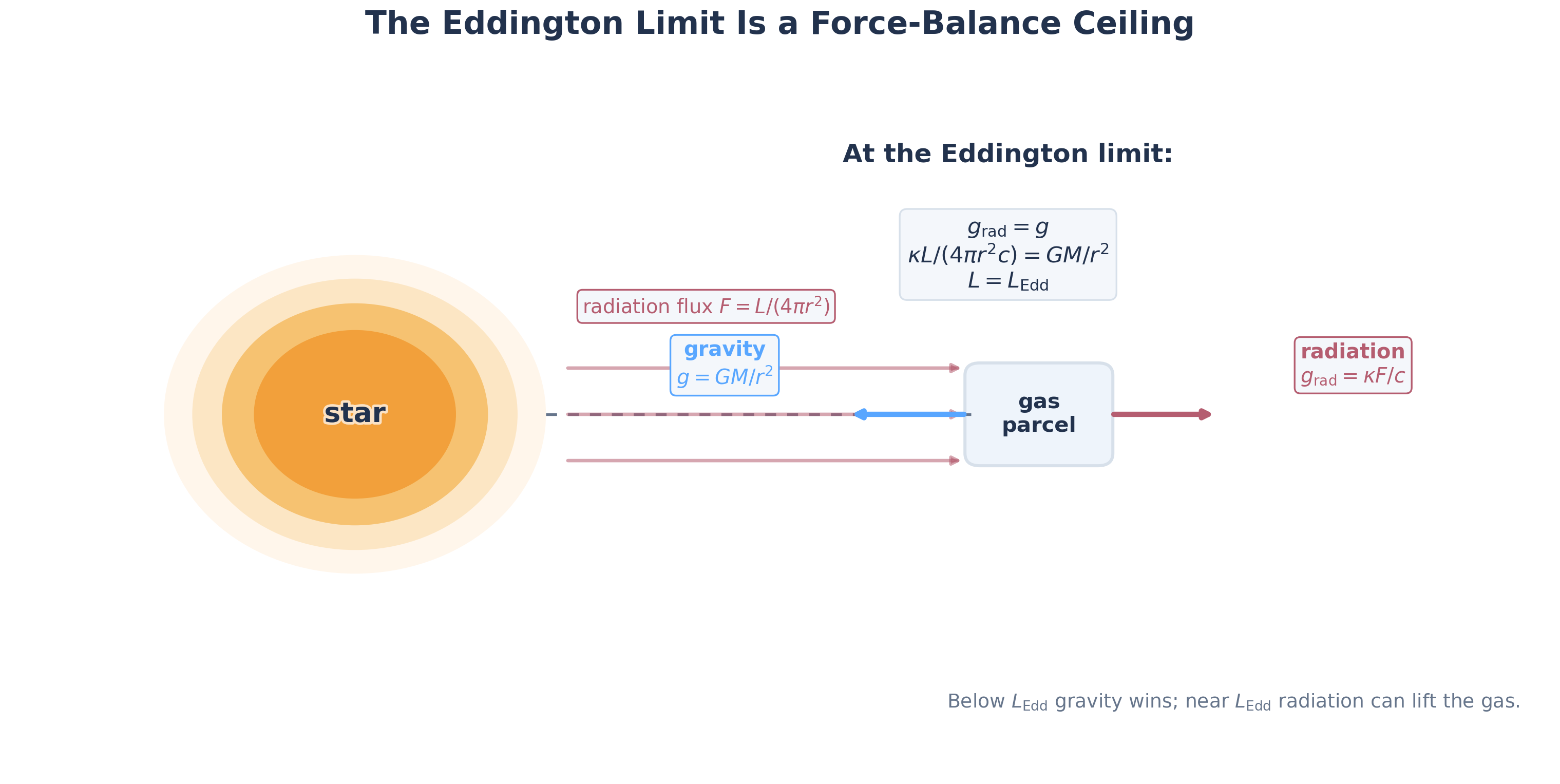
This result comes from a direct force balance: radiation pushes outward because photons transfer momentum to matter, while gravity pulls inward.

① Write the balance. Per unit mass, the outward radiative force is $f_\text{rad} = \kappa F/c$ with flux $F = L/(4\pi r^2)$ , and the inward gravitational force is $f_\text{grav} = GM/r^2$ . Here $\kappa$ is the opacity in $\text{cm}^2/\text{g}$ and $c$ is the speed of light. Set them equal:

\frac{\kappa L}{4 \pi r^2 c} = \frac{GM}{r^2}.

② Solve — the size cancels. The $r^2$ drops out of both sides (just as the radius dropped out of the minimum-mass temperature), so the ceiling depends on total mass and luminosity, not on where we evaluate the balance:

L_{\text{Edd}} = \frac{4 \pi GMc}{\kappa}.

③ Read off the constants. The ceiling is built from $G$ (gravity), $c$ (relativity), and $\kappa$ (the opacity microphysics — in hot stars, electron scattering). The Eddington luminosity is not a mysterious formula to memorize: it is simply the luminosity at which radiation force competes directly with gravity.

Schematic showing a star on the left and a gas parcel in the envelope on the right. An inward arrow labeled gravity points from the parcel toward the star, and an outward arrow labeled radiative acceleration points away from the star. Text boxes show g equals GM over r squared, g_rad equals kappa L over four pi r squared c, and the Eddington limit condition g_rad equals g. — Figure 2The Eddington luminosity comes from a force balance on a gas parcel. Gravity pulls inward with g = GM/r^2, while radiation pushes outward with g_rad = kappa L / (4 pi r^2 c). Setting them equal gives the luminosity at which radiation pressure competes directly with gravity.ASTR 201 (generated)

For electron-scattering opacity ( $\kappa \approx 0.34~\text{cm}^2/\text{g}$ ), this gives

\frac{L_\text{Edd}}{L_\odot} \approx 3.8 \times 10^4 \left(\frac{M}{M_\odot}\right),

so the Eddington luminosity scales linearly with mass: $L_\text{Edd} \propto M$ .

Numeric answer

Compute the Eddington luminosity of a $10\,M_\odot$ star from scratch, using $L_\text{Edd} = 4\pi GMc/\kappa$ with electron-scattering opacity $\kappa = 0.34~\text{cm}^2\text{g}^{-1}$ (everything CGS: $G = 6.67\times10^{-8}$ , $c = 3\times10^{10}$ , $M_\odot = 1.99\times10^{33}~\text{g}$ ). Enter your answer in $\text{erg}\,\text{s}^{-1}$ .

Your answer

Why There’s a Maximum Mass

For moderate-mass main-sequence stars, the luminosity follows the mass-luminosity relation from Module 3 (the stellar blueprint):

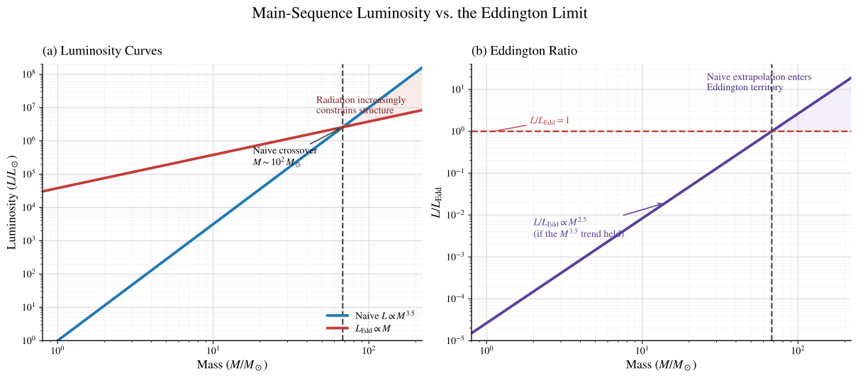
If you naively extrapolate that moderate-mass trend, luminosity rises much faster than the Eddington limit.

$M/M_\odot$	Naive $L/L_\odot$ ( $\propto M^{3.5}$ )	$L_\text{Edd}/L_\odot$ ( $\propto M$ )	Naive $L/L_\text{Edd}$
1	1	$3.8 \times 10^4$	$2.6 \times 10^{-5}$
10	$3{,}200$	$3.8 \times 10^5$	$8.4 \times 10^{-3}$
50	$8.8 \times 10^5$	$1.9 \times 10^6$	0.46
100	$10^7$	$3.8 \times 10^6$	2.6

This table is useful because it shows why an upper limit appears at all. If luminosity rises faster than the Eddington limit, radiation becomes increasingly important. But this table is only an order-of-magnitude guide: at the highest masses, the mass-luminosity relation flattens, radiation pressure reshapes the interior, and the star responds by driving powerful radiation-driven winds that strip mass from the surface.

Two-panel white-background log-log figure. Left panel plots stellar luminosity versus mass with a blue curve labeled naive main sequence L proportional to M to the 3.5 and a red curve labeled Eddington limit proportional to M. A dashed vertical line marks a crossover near 100 solar masses, and a shaded region indicates where radiation increasingly constrains structure. Right panel plots the ratio L over L Edd versus mass with a horizontal line at 1 and a purple curve that rises steeply toward and past unity near the same mass scale. — Figure 3The naive main-sequence relation rises much more steeply than the Eddington limit. In the left panel the two curves approach each other near M ~ 100 solar masses. In the right panel the ratio L/L_Edd rises as M^2.5 if the moderate-mass trend is extrapolated blindly, which is why an upper-mass scale appears instead of arbitrarily luminous stable stars.ASTR 201 (generated)

Finding the Maximum Mass

The crossover occurs when $L = L_\text{Edd}$ :

\left(\frac{M}{M_\odot}\right)^{3.5} = 3.8 \times 10^4 \left(\frac{M}{M_\odot}\right) \;\Longrightarrow\; \left(\frac{M}{M_\odot}\right)^{2.5} = 3.8 \times 10^4,

\frac{M}{M_\odot} = (3.8 \times 10^4)^{1/2.5} = (3.8 \times 10^4)^{0.4} \approx 70.

A naive crossover estimate therefore gives an upper-mass scale of order

\boxed{M_\text{max} \sim 70\,M_\odot}.

This is only a rough lower estimate. The naive $L \propto M^{3.5}$ overestimates the luminosity at very high mass, so it makes luminosity catch the Eddington line too early; the real mass-luminosity relation flattens (closer to $L \propto M^{1\text{–}2}$ near the Eddington regime), which pushes the true ceiling higher. Stars up to roughly $\sim 150$ – $200\,M_\odot$ have been observed. The lesson is the scale — tens to a couple hundred solar masses — not a hard wall at any single number, and certainly not a number the simple crossover pins down precisely.

Numeric answer

The most massive known star, R136a1, has a current mass of $\sim 170\,M_\odot$ and a luminosity of $\sim 4 \times 10^6\,L_\odot$ . Using $L_\text{Edd} = 3.8 \times 10^4\,(M/M_\odot)\,L_\odot$ , calculate its Eddington ratio $L/L_\text{Edd}$ .

Your answer

Why the Maximum Mass is Also Set by Constants

Just as the minimum mass depends on fundamental constants, so does the maximum mass. The Eddington limit comes from balancing radiation force ( $L\kappa/(4\pi r^2 c)$ ) against gravity ( $GM/r^2$ ), so the upper-mass scale depends on gravity through $G$ , on relativity through $c$ , and on opacity physics through $\kappa$ (which in hot stars is tied to electron scattering).

Quick check

Both walls are “written in the constants” — but in different constants.

(a) Which fundamental constants set the minimum mass, and which set the maximum mass? Which players do the two limits share, and which are unique to each?
(b) The minimum-mass scale is $M_0 = (\hbar c/G)^{3/2}/m_p^2$ . If $\hbar$ were somehow larger, would the minimum stellar mass go up or down? Reason physically, not just from the formula.

The More You Know: Enrichment: Beyond the Eddington Limit — Pair-Instability Supernovae

Very massive stars ( $M \gtrsim 130\,M_\odot$ at the end of their lives) face an even more dramatic fate. In their extremely hot cores ( $T \gtrsim 10^9~\text{K}$ ), photons become energetic enough to spontaneously create electron-positron pairs ( $\gamma \rightarrow e^+ + e^-$ ). This process removes photons that were providing radiation pressure support. The core partially collapses, triggers explosive oxygen and silicon burning, and the resulting thermonuclear explosion can be powerful enough to completely obliterate the star — leaving no remnant at all.

These pair-instability supernovae are predicted to be among the most energetic explosions in the universe, outshining entire galaxies for weeks. They may have been common among the first generation of stars (which formed from pristine hydrogen and helium, with no metals to increase opacity and drive winds). Several candidate events have been observed (e.g., SN 2007bi), though confirmation remains challenging.

This is another case where quantum mechanics (pair creation from $E = mc^2$ ) has dramatic astrophysical consequences — a theme that runs through all of Module 4.