The Boundaries of Stardom

By the end of this reading, you will be able to:

• Explain

  why there is a minimum mass for hydrogen fusion ($\sim 0.08\,M_\odot$) using quantum confinement and electron degeneracy

• State

  the Heisenberg uncertainty principle and explain how confining particles gives them momentum

• Explain

  why there is a maximum stellar mass ($\sim 100$–$150\,M_\odot$) set by the Eddington luminosity

• Describe

  what brown dwarfs are and why they fail to sustain hydrogen fusion

• Calculate

  the Eddington luminosity and compare it to a main-sequence luminosity estimate

• Explain

  how both mass limits depend on fundamental constants of nature

Guiding question: why can’t a star be any mass it wants? Nature imposes a floor and a ceiling — and both are written into fundamental constants.

The main sequence has edges. You can’t build a star of any mass — nature imposes two boundaries, each enforced by different physics. At the bottom, quantum mechanics prevents continued contraction before the core gets hot enough for sustained fusion. At the top, radiation becomes so important that the most massive stars drive extreme winds and approach a luminosity ceiling. Both limits depend on fundamental constants, which means the range of stellar masses is written into the laws of physics.

Part 1: The Mystery at the Bottom

Observationally, the main sequence ends near $\sim 0.08\,M_\odot$. Below that boundary, we find brown dwarfs: objects that form like stars but cool and fade instead of sustaining hydrogen fusion. The puzzle is not whether gravity tries to compress them. It does. The puzzle is why gravity fails before fusion ignition.

Brown dwarf

A substellar object below the hydrogen-burning minimum mass ($\sim 0.08\,M_\odot \approx 80\,M_\text{Jupiter}$) in which electron degeneracy halts contraction before the core reaches sustained hydrogen-fusion temperatures. It glows faintly from gravitational (Kelvin-Helmholtz) contraction and brief deuterium burning, then cools and fades.

Why Can’t Small Stars Get Hot Enough?

In Module 3 (hydrostatic equilibrium), we derived the core-temperature estimate from the virial theorem:

At first glance, this seems to say that any mass can reach any temperature — just make $R$ small enough. A contracting protostar should get hotter and hotter until fusion ignites. And indeed, for solar-mass stars, this works: gravitational contraction heats the core to $\sim 15~\text{MK}$ and fusion begins.

But there’s a hidden assumption: we treated the gas as classical particles — tiny billiard balls with well-defined positions and velocities. This works beautifully for the Sun, where the interparticle spacing is much larger than the particles’ quantum wavelengths. But as the star contracts and the density rises, the particles get squeezed closer and closer together. Eventually, a fundamental limit of quantum mechanics kicks in.

The de Broglie Wavelength Revisited

In Module 3 (nuclear fusion), we introduced the de Broglie wavelength — the quantum wavelength associated with any particle:

For a particle with thermal energy $\frac{1}{2}mv^2 \sim \frac{3}{2}k_BT$, the typical velocity is $v \sim \sqrt{3k_BT/m}$, and the de Broglie wavelength becomes $\lambda_\text{dB} \sim h/\sqrt{3mk_BT}$.

At the Sun’s core ($T_c \sim 1.5 \times 10^7~\text{K}$), the de Broglie wavelength of a proton is:

$$\lambda_\text{dB} \sim \frac{6.63 \times 10^{-27}~\text{erg}\cdot\text{s}} {\sqrt{3 \times 1.67 \times 10^{-24}~\text{g} \times 1.38 \times 10^{-16}~\text{erg}\,\text{K}^{-1} \times 1.5 \times 10^7~\text{K}}} \approx 6.5 \times 10^{-11}~\text{cm}$$

The average interparticle spacing in the solar core is:

$$d \sim n^{-1/3} \sim \left(\frac{\rho}{m_p}\right)^{-1/3} \sim \left(\frac{150~\text{g}\,\text{cm}^{-3}}{1.67 \times 10^{-24}~\text{g}}\right)^{-1/3} \sim 2 \times 10^{-9}~\text{cm}$$

So in the Sun, $\lambda_\text{dB} \approx 6.5 \times 10^{-11}~\text{cm} \ll d \sim 2 \times 10^{-9}~\text{cm}$ — the quantum wavelength is about $30\times$ smaller than the particle spacing. The particles “fit” comfortably as classical objects. Quantum mechanics plays a role in nuclear reactions (tunneling), but the gas behavior is classical.

This proton calculation is an intuition check, not the actual brown-dwarf support mechanism. Brown dwarfs are supported by electron degeneracy pressure. Because electrons are much lighter than protons, they acquire much larger quantum wavelengths and become degenerate first. We can make that statement more explicit. Start from $\lambda_\text{dB} = h/(mv)$. For particles in the same thermal environment, $v \sim \sqrt{3k_B T/m}$, so

$$\lambda_\text{dB} \sim \frac{h}{m\sqrt{3k_B T/m}} \propto \frac{1}{\sqrt{m}}.$$

Therefore,

$$\frac{\lambda_e}{\lambda_p} \sim \sqrt{\frac{m_p}{m_e}} \approx \sqrt{1836} \approx 43.$$

So at the same temperature, electron quantum wavelengths are tens of times larger than proton quantum wavelengths. That is why electrons reach the overlap condition first and become degenerate first.

When Quantum Effects Take Over

Now imagine a lower-mass object — say $0.05\,M_\odot$ — trying to contract toward fusion ignition. As it contracts:

• $\rho$ increases, so the interparticle spacing $d \propto \rho^{-1/3}$ decreases,
• $T$ increases (virial theorem), so $\lambda_\text{dB} \propto T^{-1/2}$ decreases — but more slowly than $d$.

Eventually, the electron de Broglie wavelength becomes comparable to the electron spacing. At that point, the gas is no longer classical. Electron wavefunctions overlap, and quantum mechanics fundamentally changes the gas’s behavior. The critical condition is

$$\lambda_{\text{dB},e} \sim n_e^{-1/3}.$$

When this condition is reached, the electrons become degenerate — a state where quantum mechanical effects dominate the pressure. We’ll explore degeneracy pressure fully in Reading 3 (degeneracy and the Chandrasekhar limit), but the key insight is this: degenerate matter resists further compression even without any thermal energy. Quantum mechanics generates pressure at zero temperature.

Quick check

In the Sun’s core, we found $\lambda_\text{dB}/d \sim 1/30$. Why does this ratio tell us the solar core is safely classical? What would happen if a star contracted enough that $\lambda_\text{dB}/d \sim 1$?

Part 2: The Heisenberg Uncertainty Principle

Confinement Creates Momentum

The de Broglie wavelength argument tells us when quantum effects matter. But why does confining particles generate pressure? The answer is one of the deepest results in quantum mechanics: the Heisenberg uncertainty principle.

Here $\Delta x$ is the uncertainty in position and $\Delta p$ is the uncertainty in momentum, and the reduced Planck constant is $\hbar = h/2\pi = 1.055 \times 10^{-27}~\text{erg}\cdot\text{s}$.

Heisenberg uncertainty principle

The quantum law $\Delta x \cdot \Delta p \geq \hbar/2$: a particle’s position and momentum cannot both be sharply defined. Confining a particle to a region of size $\Delta x$ forces a minimum momentum $p \sim \hbar/\Delta x$ — so compression alone gives particles momentum, and therefore pressure, even at zero temperature.

What this says: you cannot simultaneously know a particle’s exact position and exact momentum. The more precisely you confine a particle (smaller $\Delta x$), the larger its momentum uncertainty ($\Delta p$) must be — and therefore the faster the particle moves. This is not a limitation of measurement technology. It is a fundamental property of nature. A particle confined to a region of size $\Delta x$ must have a minimum momentum of $p_\text{min} \sim \hbar/\Delta x$.

To get the corresponding kinetic-energy scale, substitute that momentum into the non-relativistic kinetic-energy relation $E \sim p^2/(2m)$. Then

$$E_\text{min} \sim \frac{1}{2m}\left(\frac{\hbar}{\Delta x}\right)^2 \sim \frac{\hbar^2}{2m(\Delta x)^2}.$$

Now set the confinement scale by the interparticle spacing, $\Delta x \sim d \sim n^{-1/3}$. Then

$$E_\text{min} \sim \frac{\hbar^2}{2m d^2} \propto \frac{1}{d^2} \propto n^{2/3}.$$

Compression raises the density, and higher density forces higher momentum and higher kinetic energy. That is the origin of the quantum pressure trend.

Why This Matters for Stars

In a dense stellar core, the interparticle spacing $d \sim n^{-1/3}$ sets the confinement scale. If you try to squeeze particles closer together ($\Delta x \sim d$ decreasing), the uncertainty principle forces their momenta up:

$$p \sim \frac{\hbar}{d} \sim \hbar\,n^{1/3}.$$

These fast-moving particles exert pressure — even if the temperature is zero. This is degeneracy pressure, a fundamentally quantum mechanical effect with no classical analogue. The critical insight: gravity tries to compress the star, but compression creates quantum momentum, which creates pressure that resists further compression. There’s a natural equilibrium point where gravitational squeezing balances quantum resistance.

Worked Example 1Zero-Point Energy of a Confined Electron

Problem

Suppose an electron is confined to a box of size $\Delta x = 10^{-8}~\text{cm}$ (roughly atomic scale, about 1 angstrom). What is its minimum kinetic energy?

Step·Minimum momentum from the uncertainty principle

$p_\text{min} \sim \frac{\hbar}{\Delta x} = \frac{1.055 \times 10^{-27}~\text{erg}\cdot\text{s}}{10^{-8}~\text{cm}} = 1.055 \times 10^{-19}~\text{g}\,\text{cm}/\text{s}$

Step·Minimum kinetic energy

$E_\text{min} \sim \frac{p_\text{min}^2}{2m_e} = \frac{(1.055 \times 10^{-19})^2}{2 \times 9.11 \times 10^{-28}} \sim 6 \times 10^{-12}~\text{erg} \sim 4~\text{eV}$

Dimensional check

$[E] = \dfrac{[\text{g}\,\text{cm}/\text{s}]^2}{\text{g}} = \dfrac{\text{g}^2\,\text{cm}^2\,\text{s}^{-2}}{\text{g}} = \text{g}\,\text{cm}^2\,\text{s}^{-2} = \text{erg}$ ✓.

Result

This is the zero-point energy — the minimum kinetic energy an electron must have when confined to atomic scales. The number matters less than the pattern: tighter confinement forces larger momentum and therefore larger kinetic energy. That same logic is what makes degeneracy pressure rise in dense stellar matter.

Numeric answer

If you squeeze the box to half its size ($\Delta x \rightarrow \Delta x/2$), by what factor does the minimum kinetic energy $E_\text{min}$ increase? Enter the multiplicative factor.

Your answer

Part 3: The Minimum Stellar Mass

The Physical Argument

For a collapsing gas cloud to become a hydrogen-burning star, its core must reach $T_c \sim 3 \times 10^6~\text{K}$ — the minimum temperature for pp-chain fusion to sustain energy losses. (This is lower than the Sun’s $15~\text{MK}$ because fusion rates have a steep temperature dependence — even a slow trickle of fusion at $3~\text{MK}$ can sustain a very low-luminosity star.)

As the protostar contracts, the virial theorem tells us the core heats up: $T_c \propto M/R$. But contraction also increases the density, and eventually the electrons become degenerate. Once that happens, the gas behaves differently:

1. Pressure no longer depends on temperature. Degeneracy pressure is set by density, not $T$. So adding heat doesn’t increase pressure — the star can’t expand in response to heating.
2. Contraction halts. Degeneracy pressure balances gravity at a specific radius, regardless of temperature.
3. The core may never get hot enough. If degeneracy kicks in before the core reaches $\sim 3 \times 10^6~\text{K}$, the star is stuck — it has a cold, dense, quantum-pressure-supported core that will never achieve sustained fusion.

The Critical Mass

The hydrogen-burning minimum mass (HBMM) depends on when degeneracy sets in relative to the fusion ignition temperature. Detailed calculations give:

Objects below this mass are brown dwarfs — failed stars that glow faintly from residual gravitational contraction energy (Kelvin-Helmholtz) and possibly brief deuterium burning, but never achieve sustained hydrogen fusion.

Why 0.08 Solar Masses? — Reading the Limit

We now have the ingredients to derive the floor, not just assert it. This is the first appearance of the move that runs through all of Module 4 — Reading the Limit.

① Write the balance. A contracting protostar carries two energies per particle, and as it shrinks at fixed mass $M$ they pull the temperature in opposite directions. Virial heating supplies a thermal energy

$$k_B T \sim \frac{GM m_p}{R} \propto \frac{1}{R},$$

while the electrons carry a quantum (Fermi) energy set by how tightly they are confined,

$$E_F \sim \frac{\hbar^2}{m_e}\,n_e^{2/3} \sim \frac{\hbar^2}{m_e}\left(\frac{M}{m_p R^3}\right)^{2/3} \propto \frac{1}{R^2}.$$

As the protostar contracts, both energies rise — but the quantum energy rises faster ($R^{-2}$ beats $R^{-1}$). So the core temperature climbs, peaks, and then falls as degeneracy takes over. The hottest the core ever gets is the moment the two energies meet, $k_B T \sim E_F$.

② Solve for the critical scale. Set them equal; the radius drops out of the temperature:

$$\frac{GM m_p}{R} \sim \frac{\hbar^2}{m_e}\left(\frac{M}{m_p R^3}\right)^{2/3} \;\Longrightarrow\; k_B T_\text{max} \sim \frac{G^2 m_e\, m_p^{8/3}}{\hbar^2}\,M^{4/3}.$$

This is the key result: the maximum core temperature a star can ever reach scales as $T_\text{max} \propto M^{4/3}$. Halve the mass and the peak temperature drops by $2^{4/3} \approx 2.5$. Light enough objects never get hot enough — they reach their peak temperature below the fusion threshold and then cool forever. The minimum mass is the one whose peak just touches the ignition temperature, $T_\text{max} = T_\text{ign}$.

③ Read off the constants. Setting $T_\text{max} = T_\text{ign}$ and solving for the mass,

$$M_\text{min} \sim \underbrace{\left(\frac{\hbar c}{G}\right)^{3/2}\frac{1}{m_p^2}}_{\textstyle M_0\,\approx\,1.8\,M_\odot}\;\left(\frac{k_B T_\text{ign}}{m_e c^2}\right)^{3/4}.$$

The floor is built from $\hbar$ (quantum mechanics), $G$ (gravity), $c$ (relativity), and the particle masses $m_p, m_e$. The leading combination $M_0 = (\hbar c/G)^{3/2}/m_p^2 \approx 1.8\,M_\odot$ is a natural stellar mass scale — and you will meet it again, almost unchanged, as the Chandrasekhar mass in Reading 3. The dimensionless factor $(k_B T_\text{ign}/m_e c^2)^{3/4}$ — the ignition temperature measured against the electron rest energy — is only a few $\times 10^{-3}$, which is why the floor sits far below that natural scale, in the brown-dwarf range. Taken literally, this stripped-down scaling lands near $\sim 10^{-2}\,M_\odot$ (we dropped numerical prefactors — the $(3\pi^2)^{2/3}$ in the Fermi energy, the electron fraction $\mu_e$, the precise ignition criterion); restoring them lifts the result to the observed $\sim 0.08\,M_\odot$. The scaling delivers the origin and the order of magnitude — which constants, and a small fraction of a solar mass — and detailed models supply the exact coefficient.

The minimum stellar mass is not a coincidence of astrophysics — it is built into the laws of physics. At the low-mass end, quantum mechanics stops gravity from finishing the job. At the high-mass end, gravity succeeds in making the star extremely luminous — but that luminosity creates a new opponent: radiation force.

Quick check

Brown dwarfs with masses $0.013$–$0.08\,M_\odot$ briefly burn deuterium ($^2\text{H} + {^1\text{H}} \rightarrow {^3\text{He}} + \gamma$) but not hydrogen. Why is the deuterium-burning threshold lower than the hydrogen-burning threshold?

Part 4: The Maximum Stellar Mass

The Eddington Limit Revisited

In Module 3 (radiation transport), we introduced the Eddington luminosity — the maximum luminosity a star can sustain in hydrostatic equilibrium. The ceiling is Reading the Limit again — a second balance, solved the same way:

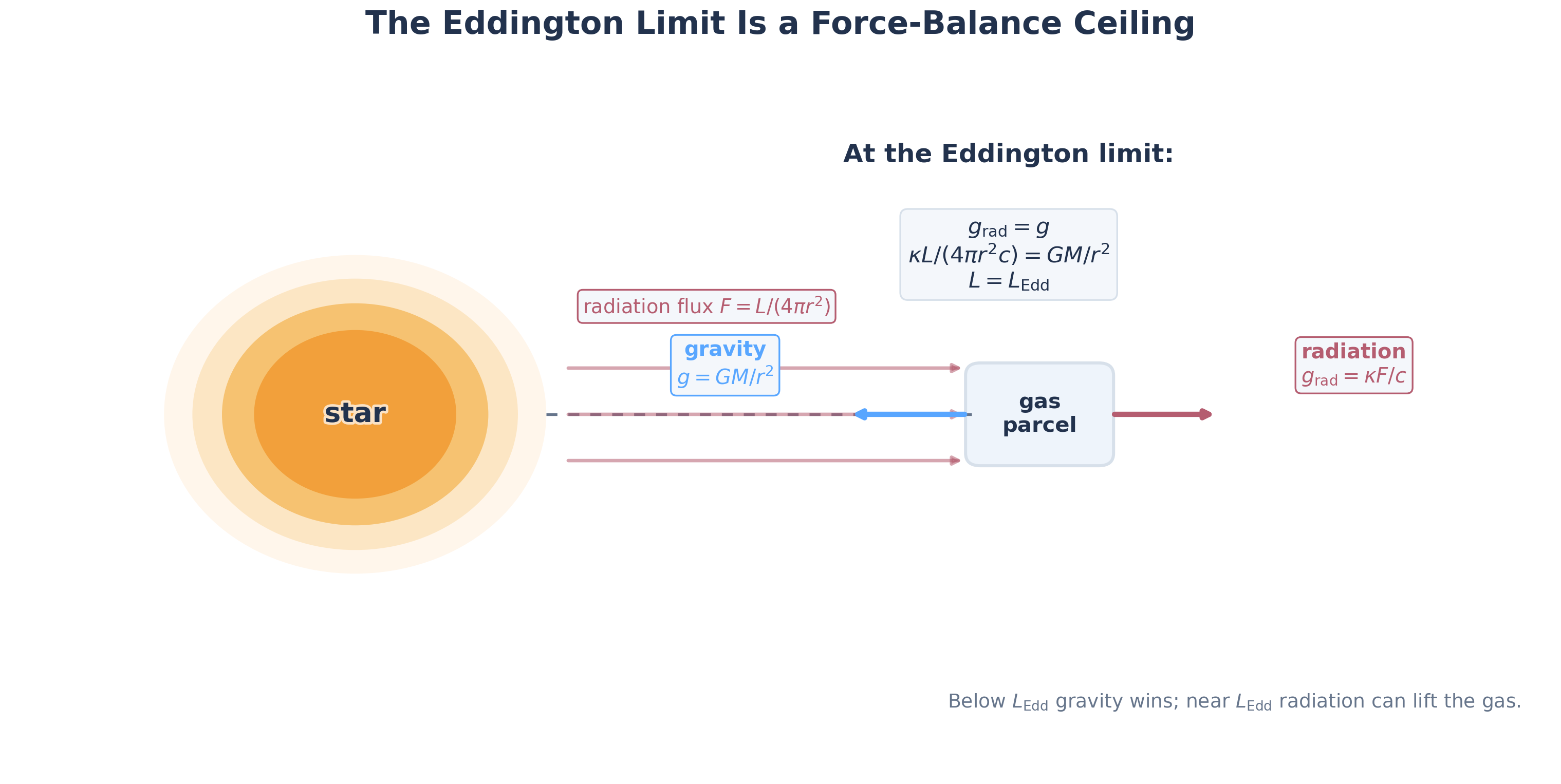
This result comes from a direct force balance: radiation pushes outward because photons transfer momentum to matter, while gravity pulls inward.

① Write the balance. Per unit mass, the outward radiative force is $f_\text{rad} = \kappa F/c$ with flux $F = L/(4\pi r^2)$, and the inward gravitational force is $f_\text{grav} = GM/r^2$. Here $\kappa$ is the opacity in $\text{cm}^2/\text{g}$ and $c$ is the speed of light. Set them equal:

$$\frac{\kappa L}{4 \pi r^2 c} = \frac{GM}{r^2}.$$

② Solve — the size cancels. The $r^2$ drops out of both sides (just as the radius dropped out of the minimum-mass temperature), so the ceiling depends on total mass and luminosity, not on where we evaluate the balance:

$$L_{\text{Edd}} = \frac{4 \pi GMc}{\kappa}.$$

③ Read off the constants. The ceiling is built from $G$ (gravity), $c$ (relativity), and $\kappa$ (the opacity microphysics — in hot stars, electron scattering). The Eddington luminosity is not a mysterious formula to memorize: it is simply the luminosity at which radiation force competes directly with gravity.

For electron-scattering opacity ($\kappa \approx 0.34~\text{cm}^2/\text{g}$), this gives

$$\frac{L_\text{Edd}}{L_\odot} \approx 3.8 \times 10^4 \left(\frac{M}{M_\odot}\right),$$

so the Eddington luminosity scales linearly with mass: $L_\text{Edd} \propto M$.

Numeric answer

Compute the Eddington luminosity of a $10\,M_\odot$ star from scratch, using $L_\text{Edd} = 4\pi GMc/\kappa$ with electron-scattering opacity $\kappa = 0.34~\text{cm}^2\text{g}^{-1}$ (everything CGS: $G = 6.67\times10^{-8}$, $c = 3\times10^{10}$, $M_\odot = 1.99\times10^{33}~\text{g}$). Enter your answer in $\text{erg}\,\text{s}^{-1}$.

Your answer

Why There’s a Maximum Mass

For moderate-mass main-sequence stars, the luminosity follows the mass-luminosity relation from Module 3 (the stellar blueprint):

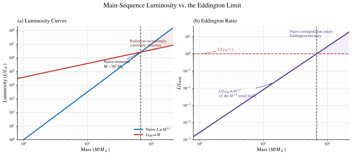
If you naively extrapolate that moderate-mass trend, luminosity rises much faster than the Eddington limit.

This table is useful because it shows why an upper limit appears at all. If luminosity rises faster than the Eddington limit, radiation becomes increasingly important. But this table is only an order-of-magnitude guide: at the highest masses, the mass-luminosity relation flattens, radiation pressure reshapes the interior, and the star responds by driving powerful radiation-driven winds that strip mass from the surface.

Finding the Maximum Mass

The crossover occurs when $L = L_\text{Edd}$:

$$\left(\frac{M}{M_\odot}\right)^{3.5} = 3.8 \times 10^4 \left(\frac{M}{M_\odot}\right) \;\Longrightarrow\; \left(\frac{M}{M_\odot}\right)^{2.5} = 3.8 \times 10^4,$$

so

$$\frac{M}{M_\odot} = (3.8 \times 10^4)^{1/2.5} = (3.8 \times 10^4)^{0.4} \approx 70.$$

A naive crossover estimate therefore gives an upper-mass scale of order

$$\boxed{M_\text{max} \sim 70\,M_\odot}.$$

This is only a rough lower estimate. The naive $L \propto M^{3.5}$ overestimates the luminosity at very high mass, so it makes luminosity catch the Eddington line too early; the real mass-luminosity relation flattens (closer to $L \propto M^{1\text{–}2}$ near the Eddington regime), which pushes the true ceiling higher. Stars up to roughly $\sim 150$–$200\,M_\odot$ have been observed. The lesson is the scale — tens to a couple hundred solar masses — not a hard wall at any single number, and certainly not a number the simple crossover pins down precisely.

Numeric answer

The most massive known star, R136a1, has a current mass of $\sim 170\,M_\odot$ and a luminosity of $\sim 4 \times 10^6\,L_\odot$. Using $L_\text{Edd} = 3.8 \times 10^4\,(M/M_\odot)\,L_\odot$, calculate its Eddington ratio $L/L_\text{Edd}$.

Your answer

Why the Maximum Mass is Also Set by Constants

Just as the minimum mass depends on fundamental constants, so does the maximum mass. The Eddington limit comes from balancing radiation force ($L\kappa/(4\pi r^2 c)$) against gravity ($GM/r^2$), so the upper-mass scale depends on gravity through $G$, on relativity through $c$, and on opacity physics through $\kappa$ (which in hot stars is tied to electron scattering).

Quick check

Both walls are “written in the constants” — but in different constants.

• (a) Which fundamental constants set the minimum mass, and which set the maximum mass? Which players do the two limits share, and which are unique to each?
• (b) The minimum-mass scale is $M_0 = (\hbar c/G)^{3/2}/m_p^2$. If $\hbar$ were somehow larger, would the minimum stellar mass go up or down? Reason physically, not just from the formula.

Part 5: The Stellar Mass Range

Nature’s Sweet Spot

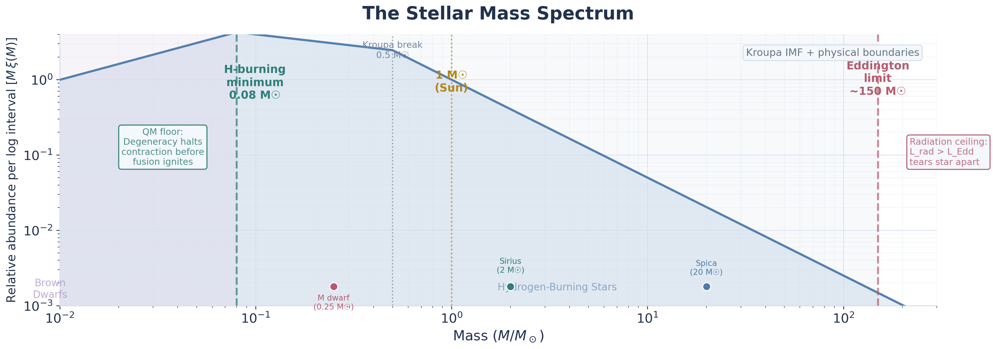
Putting the minimum and maximum together,

$$0.08\,M_\odot \lesssim M_\star \lesssim 150\,M_\odot.$$

This is a factor of $\sim 2{,}000$ in mass — which sounds like a lot, but consider:

• the range of planetary masses spans a factor of $\sim 6{,}000$ (Mercury to Jupiter),
• the range of galaxy masses spans a factor of $\sim 10^{6}$,
• the range of atomic masses spans a factor of $\sim 240$.

Stars occupy a remarkably narrow mass range, and both boundaries are set by fundamental physics:

The Mass Function: How Many Stars of Each Mass?

Not all stellar masses are equally likely. The initial mass function (IMF) — the distribution of birth masses — is observed to follow approximately a steep power law at high mass:

This is the Salpeter IMF (Edwin Salpeter, 1955), and it works best as the high-mass slope. The full IMF flattens at lower masses, but the qualitative lesson is the same: low-mass stars vastly outnumber high-mass stars.

Initial mass function

The distribution of stellar birth masses, $dN/dM$. The high-mass end follows the Salpeter power law $dN/dM \propto M^{-2.35}$; the full IMF flattens below $\sim 0.5\,M_\odot$ (Kroupa/Chabrier forms). It encodes that low-mass stars vastly outnumber high-mass stars.

The universe overwhelmingly favors making small stars — which, combined with their long lifetimes, means the most common stellar residents of the galaxy are faint, cool red dwarfs.

Numeric answer

Using the Salpeter IMF ($dN/dM \propto M^{-2.35}$), estimate how many $10\,M_\odot$ stars form for every one $100\,M_\odot$ star. Enter the ratio $N(10\,M_\odot)/N(100\,M_\odot)$.

Your answer

Reference Tables

Mass Limits at a Glance

Symbol Legend

Summary: Gravity’s Playground Has Walls

The most important ideas from this reading:

1. Quantum mechanics sets the minimum stellar mass — below $\sim 0.08\,M_\odot$, electron degeneracy halts contraction before the core reaches fusion temperatures. Objects below this limit are brown dwarfs: slowly cooling, never truly shining.
2. The Heisenberg uncertainty principle ($\Delta x \cdot \Delta p \geq \hbar/2$) means confining particles to small spaces gives them momentum — and therefore pressure. This is the origin of degeneracy pressure, which we’ll explore fully in Reading 3.
3. Radiation pressure sets the maximum stellar mass — above $\sim 100$–$150\,M_\odot$, stars approach the Eddington regime, the simple $L \propto M^{3.5}$ scaling breaks down, and strong winds make further growth difficult.
4. Both limits are built from fundamental constants — the mass range of stars is not accidental but encoded in $\hbar$, $c$, $G$, and $m_p$. The universe permits stars only in a narrow sweet spot where quantum mechanics allows fusion and radiation allows stability.

Retrieval — equation: hydrogen-burning-minimum▸

Glossary

Brown dwarf

A substellar object below the hydrogen-burning minimum mass ($\sim 0.08\,M_\odot \approx 80\,M_\text{Jupiter}$) in which electron degeneracy halts contraction before the core reaches sustained hydrogen-fusion temperatures. It glows faintly from gravitational (Kelvin-Helmholtz) contraction and brief deuterium burning, then cools and fades.

Heisenberg uncertainty principle

The quantum law $\Delta x \cdot \Delta p \geq \hbar/2$: a particle’s position and momentum cannot both be sharply defined. Confining a particle to a region of size $\Delta x$ forces a minimum momentum $p \sim \hbar/\Delta x$ — so compression alone gives particles momentum, and therefore pressure, even at zero temperature.

Initial mass function

The distribution of stellar birth masses, $dN/dM$. The high-mass end follows the Salpeter power law $dN/dM \propto M^{-2.35}$; the full IMF flattens below $\sim 0.5\,M_\odot$ (Kroupa/Chabrier forms). It encodes that low-mass stars vastly outnumber high-mass stars.