The Boundaries of Stardom

Section 5 of 6

The Stellar Mass Range

Part 5: The Stellar Mass Range

Log-log plot of stellar abundance per logarithmic mass interval versus stellar mass in solar units. The spectrum follows a schematic Kroupa IMF: it bends near 0.08 solar masses and again near 0.5 solar masses, peaks in the low-mass stellar regime, then declines steadily but continuously through the massive-star regime out to about 150 solar masses. Vertical lines mark the hydrogen-burning minimum, the Sun at 1 solar mass, the Kroupa break near 0.5 solar masses, and the Eddington upper-mass scale near 150 solar masses. Brown dwarf and hydrogen-burning star regions are lightly shaded, and sample stars including an M dwarf, Sirius, and Spica are labeled. — Figure 4The stellar mass spectrum with its quantum floor and radiation ceiling. The underlying IMF is a schematic Kroupa broken power law with slopes alpha = 0.3 below 0.08 solar masses, 1.3 from 0.08 to 0.5 solar masses, and 2.3 above 0.5 solar masses. The y-axis shows abundance per logarithmic mass interval. What to notice: the distribution bends across the brown-dwarf and low-mass-star regime, then declines steadily through the massive-star tail without dropping to zero before the Eddington upper-mass scale.ASTR 201 (generated)

Nature’s Sweet Spot

Putting the minimum and maximum together,

0.08\,M_\odot \lesssim M_\star \lesssim 150\,M_\odot.

This is a factor of $\sim 2{,}000$ in mass — which sounds like a lot, but consider:

the range of planetary masses spans a factor of $\sim 6{,}000$ (Mercury to Jupiter),
the range of galaxy masses spans a factor of $\sim 10^{6}$ ,
the range of atomic masses spans a factor of $\sim 240$ .

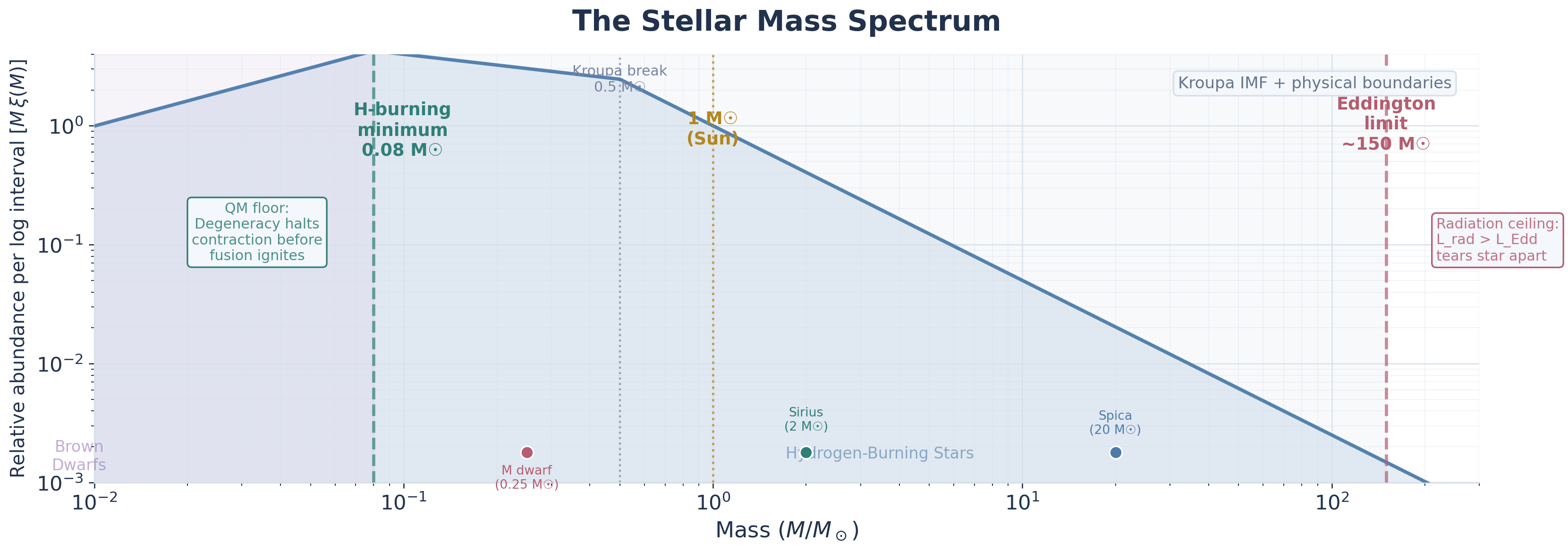
Stars occupy a remarkably narrow mass range, and both boundaries are set by fundamental physics:

Boundary	Physics	Mechanism
Minimum ( $\sim 0.08\,M_\odot$ )	Quantum mechanics	Degeneracy halts contraction before fusion ignition
Maximum ( $\sim 150\,M_\odot$ )	Radiation pressure	Stars approach the Eddington regime, drive strong winds, and struggle to grow further

The Mass Function: How Many Stars of Each Mass?

Not all stellar masses are equally likely. The initial mass function (IMF) — the distribution of birth masses — is observed to follow approximately a steep power law at high mass:

This is the Salpeter IMF (Edwin Salpeter, 1955), and it works best as the high-mass slope. The full IMF flattens at lower masses, but the qualitative lesson is the same: low-mass stars vastly outnumber high-mass stars.

Initial mass function

The distribution of stellar birth masses, $dN/dM$ . The high-mass end follows the Salpeter power law $dN/dM \propto M^{-2.35}$ ; the full IMF flattens below $\sim 0.5\,M_\odot$ (Kroupa/Chabrier forms). It encodes that low-mass stars vastly outnumber high-mass stars.

Mass range	Birth abundance
Low-mass red dwarfs	Very common
Solar-mass stars	Common
Massive O/B stars	Rare
Extreme ( $> 50\,M_\odot$ ) stars	Very rare

The universe overwhelmingly favors making small stars — which, combined with their long lifetimes, means the most common stellar residents of the galaxy are faint, cool red dwarfs.

Numeric answer

Using the Salpeter IMF ( $dN/dM \propto M^{-2.35}$ ), estimate how many $10\,M_\odot$ stars form for every one $100\,M_\odot$ star. Enter the ratio $N(10\,M_\odot)/N(100\,M_\odot)$ .

Your answer