Tools of the Trade
Complete lesson
Dimensional Analysis
By the end of this reading, you will be able to:
Why This Matters: The Challenge of Points of Light
Stars appear as mere points of light. Is that faint red glow a tiny nearby dwarf or a massive distant supergiant? We can’t visit them. We can’t weigh them directly. We can’t send a probe to measure their temperature.
So how do we know anything about them?
We need a toolkit that extracts physics from limited data. That is what this lecture provides: four methods that turn “points of light” into physical understanding.
2.1 Tool 1: Dimensional Analysis
The Smoke Detector for Physics
Here is a student’s attempt to calculate Mars’s orbital period:
Their calculator returns — of something.
Can you tell this equation is wrong without doing any calculation? Yes — and the method is called dimensional analysis.
Dimension
The physical nature of a quantity — what kind of thing it is (length, mass, time, …). Dimensions are invariant; units are conventions.
Units vs. Dimensions
Every physical quantity has two aspects. Units are human conventions: meters versus centimeters, grams versus kilograms. Dimensions are physical invariants: a length is a length, no matter what unit you measure it in.
![Split diagram contrasting UNITS (The Map) showing ruler, stopwatch, and weights labeled as 'human inventions, fungible, arbitrary' versus DIMENSIONS (The Territory) showing [L], [T], [M] symbols labeled as 'physical realities, invariant, fundamental'. Footer states physical laws must hold regardless of units used.](/astr201/figures/units-vs-dimensions-nblm.png)
We denote
| Dimension | Symbol | Examples of Units |
|---|---|---|
| Length | cm, m, AU, pc, ly | |
| Mass | g, kg, | |
| Time | s, yr, Myr |
Derived Quantities
Here is how common quantities build from the fundamental three:
![Visual equation builder showing how Mass [M], Length [L], and Time [T] combine like building blocks: Velocity = L/T → [L][T]^-1, Acceleration = velocity/time → [L][T]^-2, Force = mass × acceleration → [M][L][T]^-2, Energy = force × distance → [M][L]²[T]^-2. Includes sanity check: if your energy calculation has dimensions [M][L][T]^-1, you missed a velocity term.](/astr201/figures/fundamental-dims-nblm.png)
| Quantity | Dimensions | CGS Unit |
|---|---|---|
| Velocity | cm/s | |
| Acceleration | cm/s² | |
| Force | dyne (g cm/s²) | |
| Energy | erg (g cm²/s²) | |
| Pressure | dyne/cm² |
What are the dimensions of momentum, ?
Momentum is mass times velocity: .
The Smoke Detector Test
Here is the key idea: both sides of any valid physics equation must have the same dimensions. If you calculate a star’s mass and the answer has dimensions of time, the physics is wrong — you do not need a calculator to know something is broken.
To apply this to the student’s equation, the left side should be a period, . The right side has divided by — so first we need the dimensions of .
What Are the Dimensions of G?
Newton’s law of gravity gives us a handle on :
Let’s name every piece:
- : the gravitational force between the two bodies
- : the gravitational constant — how strong gravity is
- : the mass of the central object (e.g. a star)
- : the mass of the orbiting object (e.g. a planet)
- : the distance between the two masses
This is the equation we invert to weigh the cosmos: we never measure a gravitational force on a star directly, but its consequences — orbits, accelerations — let us solve for the masses involved. First, though, we use it for a humbler purpose: to read off the dimensions of .
We know force has dimensions . Solving Newton’s law for :
![Diagram explaining that constants like G and c are not just numbers but conversion factors. Shows c (speed of light) with dimensions [L][T]^-1 as the universal speed limit, and G (gravitational constant) derived from Newton's law with dimensions [M]^-1[L]^3[T]^-2. Highlights the inverse mass term that allows gravity to cancel mass.](/astr201/figures/physical-constants-nblm.png)
Back to the Student’s Error
Now we can check :
So the student’s equation gives
That is “time squared per length” — physically meaningless. The equation is guaranteed wrong, and we knew it before touching a calculator.
A classmate claims orbital period scales as . Could this one be right? Check its dimensions.
, and the square root gives — a time. This one survives the smoke-detector test, so it could be correct.
The Dimensional Analysis Protocol
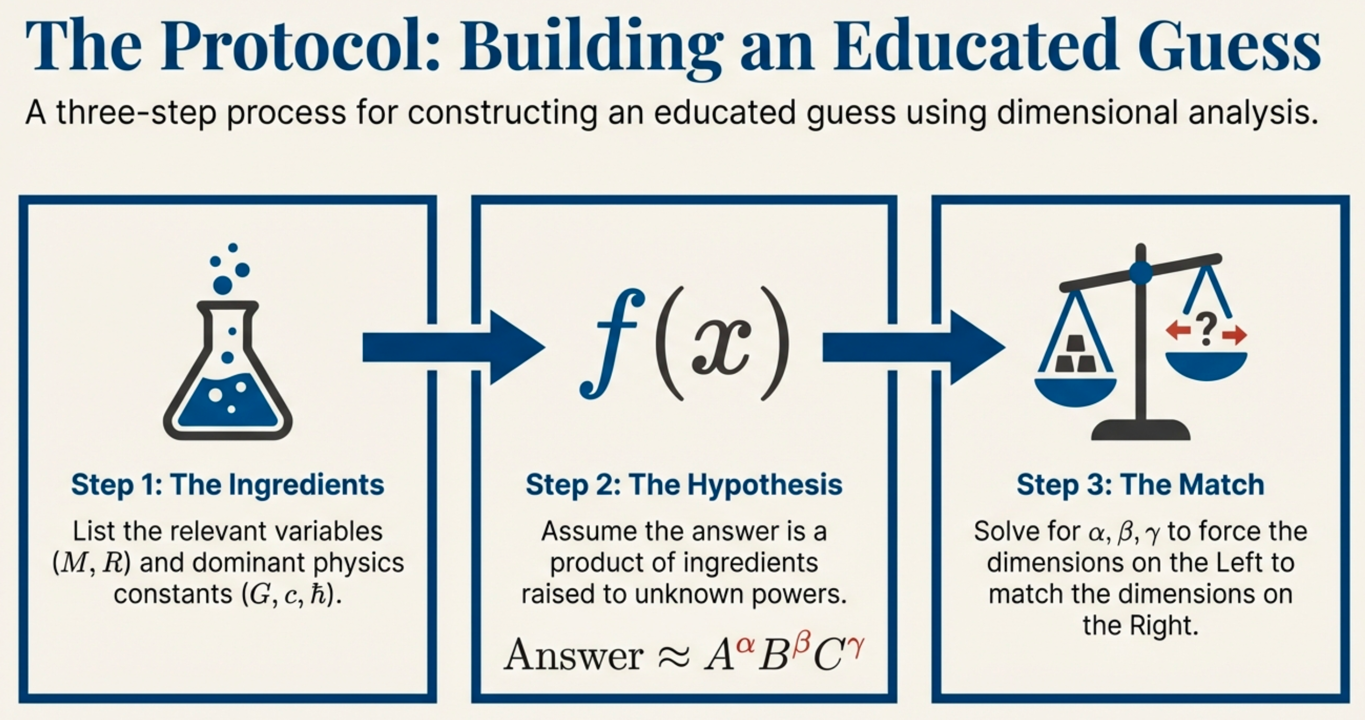
The systematic approach has five steps:
- Identify the target. What are you solving for, and what dimensions should it have?
- List the ingredients. Which quantities could the answer depend on, and what are their dimensions?
- Build a combination. Assume the answer is a product of powers:
- Match exponents. Require the dimensions to agree on both sides.
- Solve for the exponents
Worked Example: Deriving Kepler’s Third Law
Let’s derive how orbital period scales with orbital radius and central mass . The ingredients — and the target — are the dimensions we just collected:
![Diagram showing planetary orbit with star mass M and orbital radius r. Lists ingredients: Distance r with dimension [L], Star Mass M with dimension [M], Gravity G with dimension [M]^-1[L]^3[T]^-2. Target dimension: Time [T].](/astr201/figures/case-A-planetary-orbits-dimensional-analysis-1.png)
| Quantity | Dimensions |
|---|---|
| (orbital radius) | |
| (central mass) | |
| (gravitational constant) |
Problem
Find how the orbital period scales with orbital radius and central mass . The target is a time, .
StepAssume a power law
Suppose . Substituting dimensions and collecting exponents:
StepMatch exponents
Require each fundamental dimension to balance:
- Time:
- Mass:
- Length:
Dimensional check
With these exponents . Check the radicand: , so ✓ — a time, exactly as the target demands.
Result
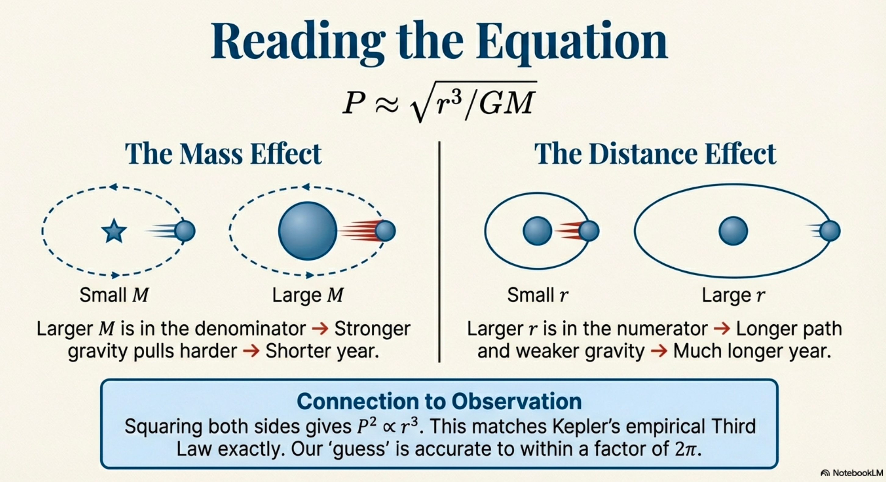
. Dimensional analysis fixes the scaling exactly but cannot supply the pure number out front; the full force-balance derivation gives .
![Three-step derivation: Step A (Kill Mass) - multiply G×M to get [L]^3[T]^-2, Step B (Kill Length) - divide by r^3 to get [T]^-2, Step C (Isolate Time) - invert and square root to get P ≈ √(r^3/GM). Result achieved with zero calculus.](/astr201/figures/case-A-planetary-orbits-dimensional-analysis-2.png)
We just derived this scaling from dimensions alone — no calculus, no orbit-solving. The registry card below records what the relationship assumes and when it breaks; the squared form makes Kepler’s empirical jump out directly.
Another Example: The Black Hole Event Horizon
What sets the “point of no return” around a black hole? We want a length scale at which gravity wins against light itself.
Event horizon
The boundary beyond which nothing — not even light — can escape a black hole’s gravitational pull. Its radius is the Schwarzschild radius.
![Diagram with black hole illustration showing curved spacetime. Goal: Find Schwarzschild radius R_sch. Ingredients: Mass M [M], Gravity G [M]^-1[L]^3[T]^-2, Speed of Light c [L][T]^-1. Target dimension: Length [L].](/astr201/figures/case-B-black-hole-dimensional-analysis-nblm-1.png)
The
| Quantity | Dimensions |
|---|---|
| (black hole mass) | |
| (gravity) | |
| (speed of light) |
Problem
Find the length scale — the horizon radius — built from , , and . The target is a length, .
StepAssume a power law
Suppose . Substituting dimensions:
StepMatch exponents
- Time:
- Mass:
- Length: , hence ,
Dimensional check
With , the combination is . Check: ✓ — a length, as required.
Result
. Dimensional analysis nails the scaling; the pure number in front needs more physics.
![Solution logic: (1) Eliminate Mass: G×M → [L]^3[T]^-2, (2) Eliminate Time: divide by c² → [L], (3) Result: R_sch ≈ GM/c². Image of accretion disk around black hole. Note: General Relativity yields exactly this scaling factor.](/astr201/figures/case-B-black-hole-dimensional-analysis-nblm-2.png)
Solving Einstein’s equations supplies the one thing dimensional analysis could not — a factor of — giving . We captured the essential physics without any of that machinery.
Using , what happens to the event horizon if you double the black hole’s mass?
Since linearly, doubling the mass doubles the horizon radius.
The Ratio Method
2.2 Tool 2: The Ratio Method
Escaping the “Big Number” Trap
The mass of the Sun is g; the mass of Earth is g. What can we do with two numbers like these?
Subtraction fails. g — still just a giant number that conveys no intuition.
Division works.
The Sun is about 333,000 times more massive than Earth. That tells you something.
Ratio method
Comparing quantities by division rather than subtraction, so that shared constants cancel and only the physically meaningful scaling survives.
The Cancellation Trick
Most physical laws are proportionalities, , where is some constant — often hiding a , a , or both. Compare two systems and the constant disappears:
The
Problem
The Sun’s radius is 109 times Earth’s, . Volume goes as . How many Earths fit inside the Sun?
StepTake the ratio
Volume scales as , so the cancels: .
Dimensional check
A ratio of like quantities is dimensionless: . The answer is a pure count, as it must be ✓.
Result
— over a million Earths. We never computed a single volume in cm³; the ratio was enough.
Scaling Intuition
The exponent in a scaling law is the physical story:
| Scaling | Physical Meaning | Example |
|---|---|---|
| Linear | Schwarzschild radius vs. mass | |
| Area scaling | Surface area, cross-section | |
| Volume scaling | Mass (at fixed density) | |
| Inverse-square | Gravity, light intensity | |
| Kepler scaling | Orbital period vs. radius |
Scaling relationship
A proportionality showing how one quantity depends on another, . The exponent carries the physics: when , small changes in the input drive large changes in the output.
When , small changes in input produce big changes in output — the heart of why a
If you double a planet’s orbital radius, by what factor does its orbital period increase?
Using , doubling gives — the period grows by about a factor of 2.8.
Applying Ratios: Mars’s Orbital Period
Kepler’s Third Law, written as a ratio against Earth as the reference, sheds every constant:
Mars orbits at AU. Substituting, , so . We predict years; the measured value is 1.88 years — excellent agreement, with no and no heavy calculation.
Jupiter orbits at 5.2 AU. Estimate its orbital period.
, so years. The measured value is 11.9 years.
Unit Conversions
2.3 Tool 3: Unit Conversions
Why Astronomers Use CGS
Astronomy runs on the CGS system — centimeter, gram, second — not the SI system you met in intro physics.
| Base Unit | CGS | SI |
|---|---|---|
| Length | cm | m |
| Mass | g | kg |
| Time | s | s |
The derived units differ too: energy in erg (not joule), force in dyne (not newton), power in erg/s (not watt).
CGS
The centimeter–gram–second system of units, standard throughout astrophysics. Derived units include the erg (energy) and dyne (force).
DigressionWhy CGS stuck
CGS became the astronomical standard in the 19th century and never left. One practical payoff: stellar luminosities and masses come out with comparable exponents — the Sun’s luminosity is erg/s, conveniently close to its mass g.
We will work in
Scientific Notation: The Language of Extremes
Astronomical numbers span more than 40 orders of magnitude, so we write them as : a coefficient between 1 and 10, times a power of ten. Positive means a big number; negative , a small one.
The exponent rules are the whole game:
| Operation | Rule | Example |
|---|---|---|
| Multiplication | Add exponents | |
| Division | Subtract exponents | |
| Powers | Multiply exponents |
Scientific notation
Expressing a number as with . Arithmetic reduces to adding, subtracting, or multiplying the exponents.
Simplify using
Divide coefficients, subtract exponents: .
SI Prefixes You’ll Use
| Prefix | Symbol | Power | Astronomy Example |
|---|---|---|---|
| giga | G | GHz (radio frequencies) | |
| mega | M | Mpc (galaxy distances) | |
| kilo | k | km, kpc | |
| centi | c | cm (the CGS base) | |
| milli | m | mm | |
| micro | μ | μm (infrared) | |
| nano | n | nm (visible light) |
The Conversion Method: Multiplying by 1
The trick is to write every conversion as a fraction equal to 1. Since ,
Multiplying by 1 never changes the physics — only how the number is written. Chain these unit-fractions so the units you don’t want cancel.
Problem
Convert Earth’s orbital speed, 30 km/s, to cm/s.
StepSet up unit-fractions equal to 1
and .
StepChain them so km and m cancel
.
Dimensional check
The km cancels against km and m against m, leaving only cm/s — a speed, as required ✓.
Result
.
Problem
The Sun’s luminosity is W. Express it in CGS (erg/s).
StepRecall the bridging conversions
and .
StepSubstitute
.
Dimensional check
Joules cancel against the erg/J factor, leaving erg/s — a power ✓.
Result
.
Convert 1 AU ( cm) to kilometers.
.
Key CGS Values to Memorize
| Quantity | CGS Value |
|---|---|
| 1 parsec | cm |
| 1 AU | cm |
| Solar mass | g |
| Solar radius | cm |
| Solar luminosity | erg/s |
| Speed of light | cm/s |
| Gravitational constant | cm³ g⁻¹ s⁻² |
Order-of-Magnitude Estimation
2.4 Tool 4: Order-of-Magnitude Estimation
You Already Do This
“Can I drive there before dinner?” You estimate: distance about 50 miles, speed about 50 mph, time about 1 hour. No calculator, and good enough. That is order-of-magnitude reasoning — and it is essential in astronomy.
Why It’s Essential
Astronomical numbers span more than 40 orders of magnitude:
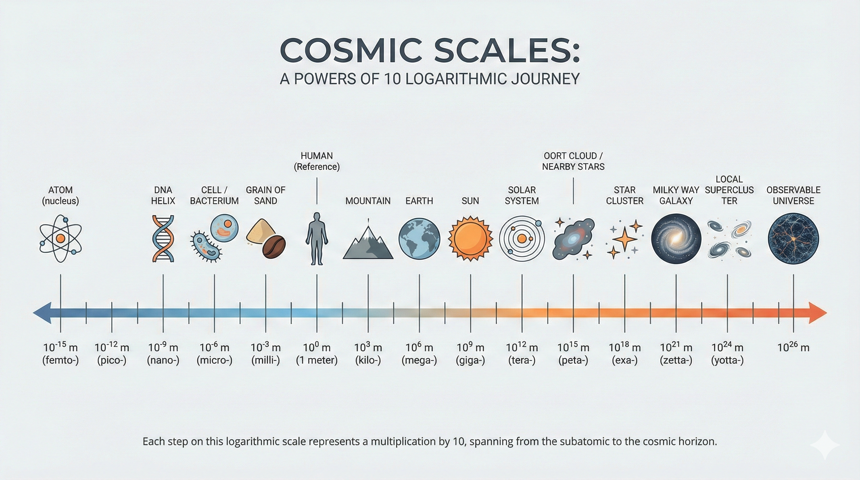
| Scale | Size (cm) | What |
|---|---|---|
| Atomic nucleus | Where fusion happens | |
| Visible wavelength | What we detect | |
| Solar radius | A typical star | |
| 1 parsec | Distance scale | |
| Observable universe | Cosmic horizon |
Exact precision can hide the physics. Off by a factor of 2? A triumph. Off by ? Something is fundamentally broken.
Order of magnitude
A power of 10. Two quantities are “within an order of magnitude” of each other when their ratio falls between 0.1 and 10.
The “Rule of 3”
When estimating, collapse each coefficient to the nearer power of ten: a coefficient below 3 rounds down to 1; above 3, up to 10. So and . Working to an
The Universe’s “Phone Number”
Here is a mnemonic for cosmic scales — the number 555-711-2555, where each digit is a number of factors of ten:
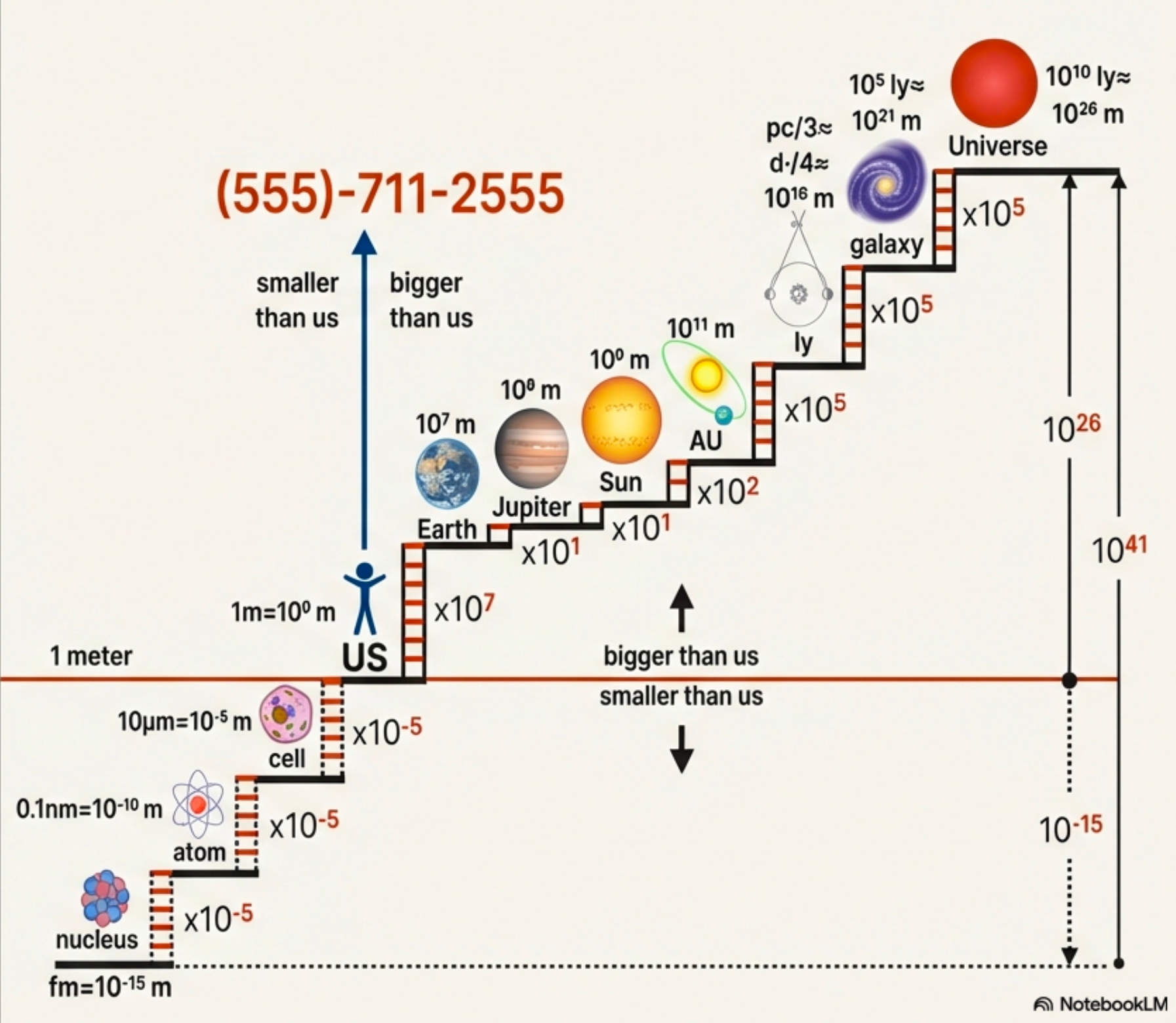
- 555 (area code) — three steps down from human scale: human → cells (), cells → atoms (), atoms → nucleus ().
- 711 (exchange) — solar-system scales: human → Earth (), Earth → Jupiter (), Jupiter → Sun ().
- 2555 (subscriber) — the cosmos: Sun → 1 AU (), AU → nearest stars (), nearest stars → Milky Way (), Milky Way → observable universe ().
A Classic Fermi Problem: Piano Tuners in Chicago
How many piano tuners work in Chicago? Estimate the pieces and chain them: population , roughly one piano per ten households gives pianos, each tuned about once a year, and one tuner handles tunings a year. Then
A reasonable ballpark, with no exact data anywhere.
Fermi estimation
Order-of-magnitude estimation that chains together rough guesses for unknown quantities to reach a defensible ballpark for something you could never look up directly.
This is
Problem
We claimed a black hole has km. Verify the order of magnitude with , rounding every input.
StepRound the ingredients (CGS)
, g, cm/s.
StepCombine
.
Dimensional check
The combination is , whose dimensions we already showed are — so the result is a length ✓.
Result
km against an exact 3 km — off by a factor of 3, i.e. within an order of magnitude. That is OOM success.
Estimate the Schwarzschild radius of Sgr A*, the Milky Way’s central black hole, with mass .
Since , scale from the value: km — about 17 solar radii, or roughly 0.08 AU, well inside Mercury’s orbit.
Connecting the Toolkit
2.5 Connecting the Toolkit
The Problem-Solving Flow
The four tools are not rivals — they work in sequence:
- Dimensional analysis: is this equation even physically valid?
- Ratio method: how does this compare to something I already know?
- Unit conversion: what is the numeric value in CGS?
- Order-of-magnitude check: does the answer make sense?
Dimensional analysis
The technique of checking or deriving relationships by requiring the dimensions on both sides of an equation to match. It verifies validity and recovers scaling laws — but never the pure numerical prefactor.
Run them together and your reasoning becomes hard to fool:
A Complete Workflow
Problem
Estimate the light-crossing time of the Milky Way, using all four tools in one pass.
StepSet up — and dimension-check
Time is distance over speed, .
Dimensional check
✓ — the setup yields a time before we touch a single number.
StepIdentify values
Milky Way diameter light-years; speed of light ly/yr (true by the definition of the light-year).
StepCompute by ratio
— the light-year units cancel cleanly.
StepOOM sanity check
Light crosses 1 ly in 1 yr; the galaxy is ly across; so yr is exactly the right ballpark.
Result
About 100,000 years. Converting to CGS seconds, s.
Summary: Your New Superpowers
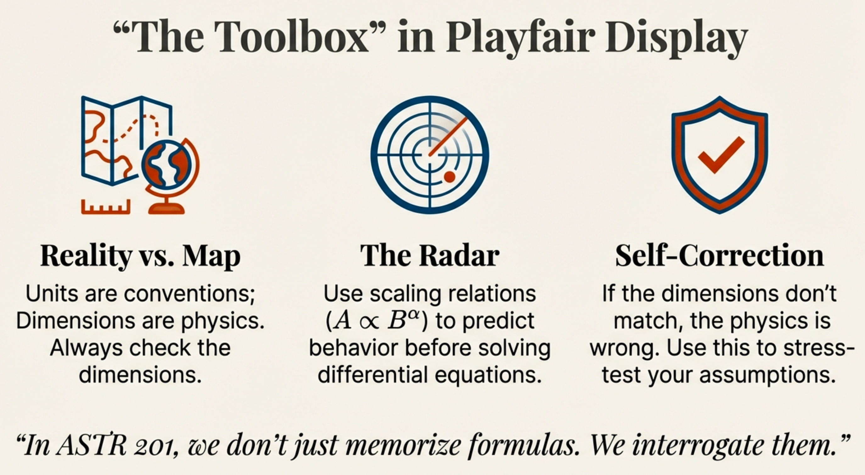
| Tool | Question It Answers | Key Insight |
|---|---|---|
| Dimensional Analysis | Is this equation physically valid? | Dimensions must match on both sides |
| Ratio Method | How does this compare to something known? | Constants cancel; the scaling tells the story |
| Unit Conversions | What is the value in CGS? | Multiply by 1; cancel units like variables |
| OOM Estimation | Does this answer make sense? | Exponents matter; coefficients are refinement |
The Workflow
- Before calculating: check dimensions.
- When comparing: use ratios.
- When computing: convert to CGS.
- After getting an answer: run an order-of-magnitude sanity check.
What You Can Now Do
With nothing but these four tools, you can derive how orbital period scales with distance (Kepler’s third law), estimate a black hole’s size from first principles via the
Schwarzschild radius
The radius of a non-rotating black hole’s event horizon, . Dimensional analysis recovers the scaling; general relativity supplies the factor of 2.
Light from the Sun takes 8.3 minutes to reach Earth. Roughly how far away is the Sun, in cm? (This is essentially the definition of 1 AU — use it as a sanity check.)
Distance speed time cm — which is 1 AU, exactly as expected.
Glossary
- CGS
The centimeter–gram–second system of units, standard throughout astrophysics. Derived units include the erg (energy) and dyne (force).
- Dimension
The physical nature of a quantity — what kind of thing it is (length, mass, time, …). Dimensions are invariant; units are conventions.
- Dimensional analysis
The technique of checking or deriving relationships by requiring the dimensions on both sides of an equation to match. It verifies validity and recovers scaling laws — but never the pure numerical prefactor.
- Event horizon
The boundary beyond which nothing — not even light — can escape a black hole’s gravitational pull. Its radius is the Schwarzschild radius.
- Fermi estimation
Order-of-magnitude estimation that chains together rough guesses for unknown quantities to reach a defensible ballpark for something you could never look up directly.
- Order of magnitude
A power of 10. Two quantities are “within an order of magnitude” of each other when their ratio falls between 0.1 and 10.
- Ratio method
Comparing quantities by division rather than subtraction, so that shared constants cancel and only the physically meaningful scaling survives.
- Scaling relationship
A proportionality showing how one quantity depends on another, . The exponent carries the physics: when , small changes in the input drive large changes in the output.
- Schwarzschild radius
The radius of a non-rotating black hole’s event horizon, . Dimensional analysis recovers the scaling; general relativity supplies the factor of 2.
- Scientific notation
Expressing a number as with . Arithmetic reduces to adding, subtracting, or multiplying the exponents.