Weighing Stars

Section 2 of 4

Binary Stars: Nature's Mass Laboratories

Part 2: Binary Stars — Nature’s Mass Laboratories

Most Stars Have Partners

One of the most important facts in stellar astronomy: roughly half of all Sun-like stars are in binary or multiple systems. For massive stars (O and B types), the binary fraction is even higher — at least 70%–90% (Sana et al. 2012). Binary stars are not rare curiosities; they are the norm.

This is fortunate, because binary orbits are the only direct way to measure stellar masses. Without binaries, the mass-luminosity relation — and much of stellar physics — would be inaccessible. So the challenge is clear: how do you weigh something you can’t touch, can’t visit, and whose mass leaves no imprint on its light? The answer is to watch it move. Astronomers have found three complementary ways to detect and exploit binary orbits, each revealing different pieces of the puzzle.

Visual Binaries: Resolved on the Sky

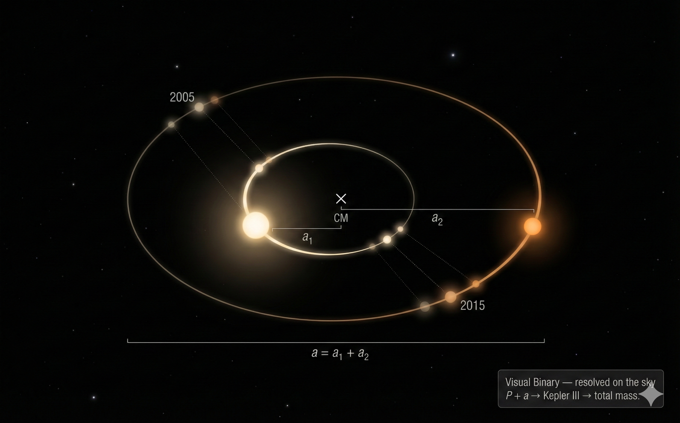
A visual binary is a pair close enough to us (and far enough apart from each other) that we can resolve both stars as separate points of light. By tracking their positions over years or decades, we map their orbits on the sky.

Visual binary

A binary whose two stars are individually resolved through a telescope, so their orbits can be traced directly on the sky over years to decades.

What visual binaries give us:

Orbital period $P$ (from watching the orbit repeat)
Angular size of the orbit on the sky (arcseconds)
If the distance is known (parallax), the angular orbit converts to a physical separation $a$ in AU or cm
From $P$ and $a$ , Kepler’s third law gives the total mass $M_1 + M_2$
If we track both stars’ orbits about the center of mass, we also get the mass ratio $M_1/M_2$

Note the critical role of distance: without parallax (Lecture 1), the angular orbit cannot be converted to a physical separation, and Kepler III cannot yield the mass. Distance — as always — is the master key. Limitation: visual binaries require wide separations (long periods, often decades to centuries) and nearby systems; they’re relatively rare in practice.

Classic example: Sirius A and Sirius B, first resolved in 1862. Sirius A is a bright A-type star ( $2.06\,M_\odot$ ); Sirius B is a white dwarf ( $1.02\,M_\odot$ ). Their period is $50.1\,\text{yr}$ and the system is only $2.64\,\text{pc}$ away.

White dwarf

The dense, Earth-sized remnant left when a low- or intermediate-mass star exhausts its fuel — about a solar mass packed into a planetary volume, shining only from stored heat.

Deep Dive: Enrichment: The Dark Companion of Sirius — A Prediction Vindicated

$Hubble Space Telescope image of the Sirius binary system. Sirius A is a brilliant overexposed white star dominating the frame with prominent diffraction spikes. Sirius B is visible as a small faint dot at lower left, separated by several arcseconds.$

Figure 2Sirius A (the brilliant overexposed star with diffraction spikes) vastly outshines Sirius B (the tiny dot at lower left). Despite a luminosity ratio of about 800:1, Sirius B has nearly half the mass of Sirius A — a white dwarf with 1.02 solar masses packed into an Earth-sized volume.NASA/ESA/HST

Figure 3The orbital path of Sirius B around Sirius A, traced over decades. Bessel predicted this companion in 1844 from the wobble of Sirius A's proper motion — the orbit was mapped long before the companion's nature was understood.Public domain

In 1844, the mathematician Friedrich Bessel noticed something strange: Sirius, the brightest star in the sky, was not moving in a straight line. Its proper motion wobbled — as if something invisible were tugging it. Bessel concluded that Sirius must have an unseen companion, and predicted its orbital period from the wobble.

This was mass measurement by gravitational influence, decades before anyone saw the companion. In 1862, telescope-maker Alvan Graham Clark spotted a faint point of light near Sirius — exactly where the orbit predicted. That dot, Sirius B, turned out to be one of the most extraordinary objects in stellar astronomy: $1.02\,M_\odot$ (nearly the Sun’s mass) crammed into a volume the size of Earth ( $R \approx 0.008\,R_\odot$ ). Its surface is about $2.5 \times 10^4\,\text{K}$ — far hotter than Sirius A — yet its luminosity is only about $0.03\,L_\odot$ . Hot but tiny: a white dwarf, the first ever identified. Bessel inferred mass from motion — exactly the strategy you are learning.

Spectroscopic Binaries: Doppler Reveals the Orbit

Most binaries are too close together and too far away to resolve visually. But we can detect them through the Doppler effect — the tool from Lecture 3.

Two-panel scientific diagram on black background. Top panel shows a binary star system at four orbital phases (0.00, 0.25, 0.50, 0.75) seen from above, with a blue-white star and an orange star orbiting their center of mass. Velocity arrows indicate approaching and receding motion at each phase, with a To Observer arrow. Bottom panel shows radial velocity versus orbital phase with two anti-phase sinusoidal curves: a blue curve with smaller amplitude K₁ and an orange curve with larger amplitude K₂. A dashed horizontal line marks the systemic velocity at zero. Annotation reads: Smaller mass → larger orbit → faster motion → larger K. — Figure 4Top: the orbital dance seen from above at four phases, with velocity arrows showing which star is approaching (blueshift) or receding (redshift). Bottom: the radial-velocity signature, two sinusoids in anti-phase. The less massive star (K2) has the larger velocity amplitude because it orbits farther from the center of mass. The mass ratio comes directly from M1/M2 = K2/K1.ASTR 201 (Gemini)

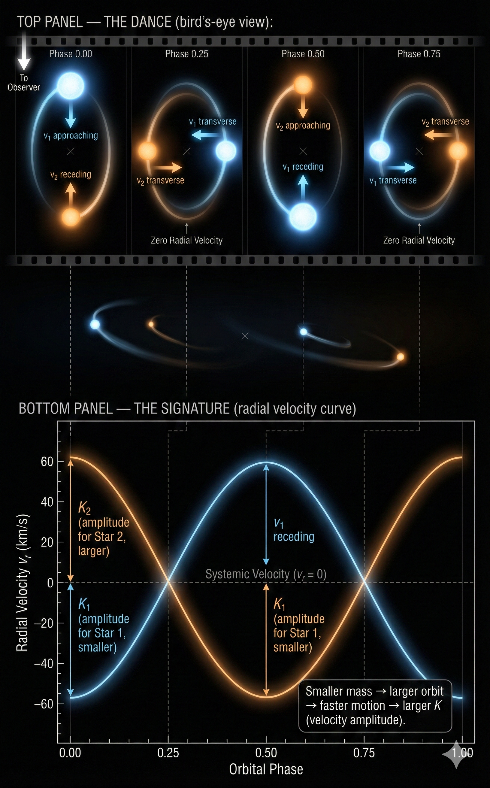
A star in a binary orbits the center of mass: during half the orbit it moves toward us, during the other half away. Its spectral lines shift back and forth — blueshifted approaching, redshifted receding — with a period equal to the orbital period. A spectroscopic binary is detected by this periodic Doppler wobble. Lecture 3 already showed a preview: the worked example of a star with Hα oscillating between $656.25\,\text{nm}$ and $656.35\,\text{nm}$ over $4.0\,\text{days}$ — that was a spectroscopic binary.

Spectroscopic binary

A binary detected from the periodic Doppler oscillation of its spectral lines as the stars orbit. It yields the period $P$ and radial-velocity amplitude $K$ even when the pair is far too close to resolve.

What spectroscopic binaries give us:

Orbital period $P$ (from the Doppler oscillation)
Radial-velocity amplitude $K$ (half the peak-to-peak velocity swing) — directly from the Doppler shift
If both stars’ lines are visible (a double-lined binary, SB2), we get $K_1$ and $K_2$ separately

Key connection to Lecture 3: the Doppler formula $\Delta\lambda/\lambda_0 = v_r/c$ converts wavelength shifts to velocities. Now we use those velocities as a function of time to trace the orbit.

Eclipsing Binaries: Light Curves Reveal Geometry

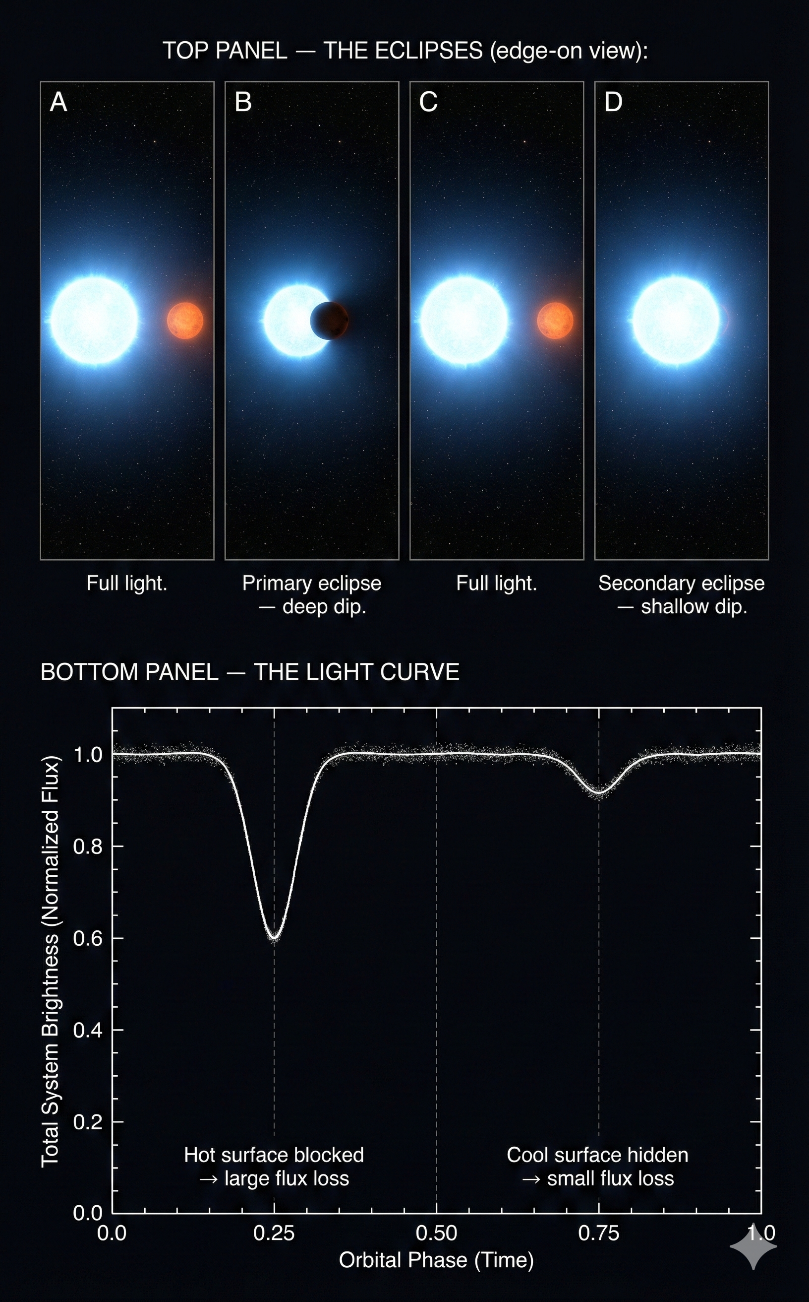
When the orbital plane is nearly edge-on, the stars periodically pass in front of each other. These are eclipsing binaries, and they produce characteristic dips in the combined light — a light curve.

Eclipsing binary

A binary whose orbit is nearly edge-on, so the stars periodically eclipse each other. The eclipses pin the inclination near $90^\circ$ and reveal the relative stellar radii and temperature ratio.

Light curve

A plot of a source’s brightness versus time. For an eclipsing binary, the spacing, depth, and shape of its dips encode the period, radii, and temperature ratio.

What eclipsing binaries give us:

Orbital period $P$ (from the spacing between eclipses)
Relative stellar radii (from the duration and shape of eclipses)
Inclination $i \approx 90^\circ$ (the orbit must be nearly edge-on for eclipses)
Temperature ratio (from the relative depths of primary and secondary eclipses)

The inclination is the prize: it removes the biggest uncertainty in spectroscopic measurements (below). The gold standard: a system that is both eclipsing and double-lined spectroscopic gives everything — period, both velocity amplitudes, inclination, and both radii — for the most precise stellar masses available (uncertainties of 1%–2%).

Classic example: Algol (β Persei), one of the first-known eclipsing binaries, dips every $2.87\,\text{days}$ as its cooler companion crosses the hot primary.

Summary: What Each Type Reveals

Binary Type	How Detected	What It Gives	What It Misses
Visual	Resolved on sky	$P$ , $a$ (with distance), mass ratio	Needs decades; nearby only
Spectroscopic	Doppler wobble	$P$ , $K_1$ (and $K_2$ if SB2)	Inclination $i$ unknown (only $v\sin i$ )
Eclipsing	Light-curve dips	$P$ , $i \approx 90^\circ$ , relative radii, $T$ ratio	Rare edge-on geometry
Eclipsing + SB2	Both	Everything: $M_1$ , $M_2$ , $R_1$ , $R_2$ , $T_1/T_2$	Rarest; edge-on and bright enough

Problem

Why can’t you measure a star’s mass from its spectrum alone?
A binary has period $30\,\text{yr}$ and the stars are resolved in a telescope. What type is it?
You observe a star whose Hα line oscillates between $656.2\,\text{nm}$ and $656.4\,\text{nm}$ every $10\,\text{days}$ . What type is it, and what can you immediately determine?

Quick check

Your lab partner says: “A star whose lines shift periodically and whose brightness dips periodically — that’s the jackpot.” Explain why this combination is so powerful. What specific problem does the eclipsing geometry solve that spectroscopy alone cannot?

Why this has to work. We need only two physics ingredients: Newtonian two-body gravity and the center-of-mass condition linking the stars. On the observation side: time variation (for $P$ ), line-of-sight velocities (for $K_1$ , $K_2$ ), and geometry (inclination $i$ ). That structure forces a specific chain: $P \to a$ ; velocity-amplitude ratio $\to$ mass ratio; total mass + mass ratio $\to$ individual masses. Once measured, there is no alternative dynamical route to $M_1$ and $M_2$ .