Weighing Stars

Complete lesson

The Hidden Variable

By the end of this reading, you will be able to:

Explain
why mass is the most fundamental stellar property and why it cannot be measured from a single, isolated star’s light alone
Describe
visual, spectroscopic, and eclipsing binary systems and explain what each reveals
Apply
Newton’s version of Kepler’s third law to determine the total mass of a binary
Use
the center-of-mass condition and radial-velocity amplitudes to determine individual masses
Interpret
the mass-luminosity relation ( $L \propto M^{3.5}$ ) and explain why it makes mass the master variable for main-sequence stars
Connect
mass measurement to the full Module 2 inference chain

Mass is the most important thing about a star — and the one thing you can’t see. Every other property — luminosity, temperature, radius, lifetime, and how a star dies — follows from mass. But mass leaves no direct imprint on a star’s light. To weigh a star, you need to catch it in a gravitational dance with a partner. Binary stars are nature’s gift to astronomers: two bodies orbiting under gravity, revealing their masses through the physics you already know.

The Big Idea

Mass determines a star’s fate — but you can’t weigh a star from its light alone.

In Lectures 1–3, you learned to measure a star’s distance, luminosity, temperature, radius, and composition from photons. But none of these tells you the most consequential property: mass. A star’s mass determines how brightly it shines, how hot its surface is, how long it lives, and how it dies. Yet mass is invisible — no spectral line, no color, no brightness measurement reveals it directly.

What you’ll gain: after this reading, you’ll know how astronomers exploit gravitational physics — binary star orbits — to measure the one property that controls all the others. And you’ll see that the resulting mass-luminosity relation is the most important empirical relation in stellar astrophysics.

Part 1: The Hidden Variable

Why Mass Matters Most

Consider two stars on the main sequence — the band where most stars spend most of their lives. One has mass $M = 0.5\,M_\odot$ ; the other $M = 10\,M_\odot$ . How do they compare?

Main sequence

The band on the H–R diagram where stars spend most of their lives in stable hydrogen-core fusion. A main-sequence star’s position is set almost entirely by its mass.

Property	$0.5\,M_\odot$ star	$10\,M_\odot$ star	Ratio
Luminosity	$\sim 0.09\,L_\odot$	$\sim 3 \times 10^3\,L_\odot$	$\sim 3 \times 10^4$
Surface temperature	$\sim 3{,}800\,\text{K}$	$\sim 2.5 \times 10^4\,\text{K}$	$\sim 7$
Radius	$\sim 0.5\,R_\odot$	$\sim 6\,R_\odot$	$\sim 12$
Main-sequence lifetime	$\sim 60\,\text{Gyr}$	$\sim 20\,\text{Myr}$	$\sim 3 \times 10^3$
Spectral type	M	B	—
Death	White dwarf	Core-collapse supernova	—

A factor of 20 in mass increases luminosity by $3 \times 10^4$ , cuts lifetime by $3 \times 10^3$ , and leads to completely different endpoints. Mass is the master variable. Change the mass, and everything else follows.

Why Mass Is Hidden

So why can’t we just “read” mass from a star’s spectrum, the way we read temperature from spectral type or composition from line wavelengths?

The problem is fundamental: mass affects a star’s light only indirectly, through its influence on internal structure. A spectrum encodes surface properties — temperature, composition, surface gravity. Mass determines those, but the mapping from mass to surface isn’t unique without a physical model connecting them. A red giant and a red dwarf can have similar surface temperatures but wildly different masses.

Put differently: luminosity, temperature, and composition are observables — encoded directly in the photons. Mass is a derived quantity — you need a physical model (or a dynamical measurement) to get it. The solution is gravity: if a star has a gravitational companion, orbital dynamics gives the mass directly, through physics you already know from Module 1.

Quick check

Recall from Module 1 (Lecture 3): Newton showed that Kepler’s third law contains the mass of the central body. For a planet orbiting the Sun we used $P^2 = 4\pi^2 r^3 / GM$ . What changes when both objects have comparable mass — like two stars orbiting each other?

Binary Stars: Nature's Mass Laboratories

Part 2: Binary Stars — Nature’s Mass Laboratories

Most Stars Have Partners

One of the most important facts in stellar astronomy: roughly half of all Sun-like stars are in binary or multiple systems. For massive stars (O and B types), the binary fraction is even higher — at least 70%–90% (Sana et al. 2012). Binary stars are not rare curiosities; they are the norm.

This is fortunate, because binary orbits are the only direct way to measure stellar masses. Without binaries, the mass-luminosity relation — and much of stellar physics — would be inaccessible. So the challenge is clear: how do you weigh something you can’t touch, can’t visit, and whose mass leaves no imprint on its light? The answer is to watch it move. Astronomers have found three complementary ways to detect and exploit binary orbits, each revealing different pieces of the puzzle.

Visual Binaries: Resolved on the Sky

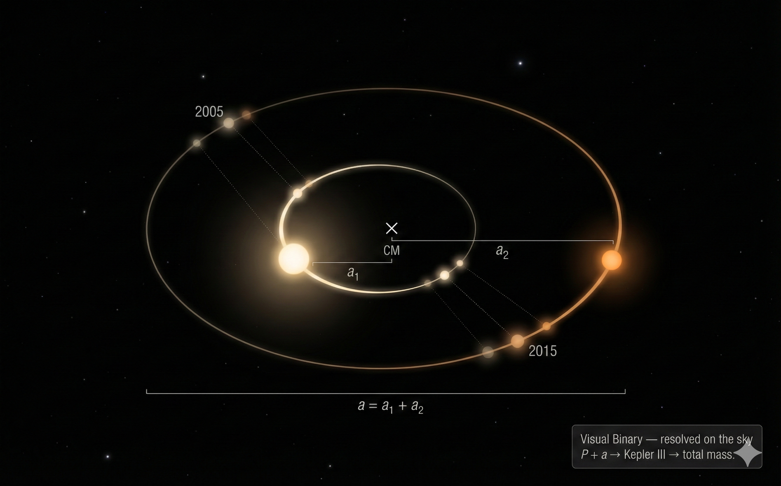
A visual binary is a pair close enough to us (and far enough apart from each other) that we can resolve both stars as separate points of light. By tracking their positions over years or decades, we map their orbits on the sky.

Visual binary

A binary whose two stars are individually resolved through a telescope, so their orbits can be traced directly on the sky over years to decades.

What visual binaries give us:

Orbital period $P$ (from watching the orbit repeat)
Angular size of the orbit on the sky (arcseconds)
If the distance is known (parallax), the angular orbit converts to a physical separation $a$ in AU or cm
From $P$ and $a$ , Kepler’s third law gives the total mass $M_1 + M_2$
If we track both stars’ orbits about the center of mass, we also get the mass ratio $M_1/M_2$

Note the critical role of distance: without parallax (Lecture 1), the angular orbit cannot be converted to a physical separation, and Kepler III cannot yield the mass. Distance — as always — is the master key. Limitation: visual binaries require wide separations (long periods, often decades to centuries) and nearby systems; they’re relatively rare in practice.

Classic example: Sirius A and Sirius B, first resolved in 1862. Sirius A is a bright A-type star ( $2.06\,M_\odot$ ); Sirius B is a white dwarf ( $1.02\,M_\odot$ ). Their period is $50.1\,\text{yr}$ and the system is only $2.64\,\text{pc}$ away.

White dwarf

The dense, Earth-sized remnant left when a low- or intermediate-mass star exhausts its fuel — about a solar mass packed into a planetary volume, shining only from stored heat.

Deep Dive: Enrichment: The Dark Companion of Sirius — A Prediction Vindicated

$Hubble Space Telescope image of the Sirius binary system. Sirius A is a brilliant overexposed white star dominating the frame with prominent diffraction spikes. Sirius B is visible as a small faint dot at lower left, separated by several arcseconds.$

Figure 2Sirius A (the brilliant overexposed star with diffraction spikes) vastly outshines Sirius B (the tiny dot at lower left). Despite a luminosity ratio of about 800:1, Sirius B has nearly half the mass of Sirius A — a white dwarf with 1.02 solar masses packed into an Earth-sized volume.NASA/ESA/HST

Figure 3The orbital path of Sirius B around Sirius A, traced over decades. Bessel predicted this companion in 1844 from the wobble of Sirius A's proper motion — the orbit was mapped long before the companion's nature was understood.Public domain

In 1844, the mathematician Friedrich Bessel noticed something strange: Sirius, the brightest star in the sky, was not moving in a straight line. Its proper motion wobbled — as if something invisible were tugging it. Bessel concluded that Sirius must have an unseen companion, and predicted its orbital period from the wobble.

This was mass measurement by gravitational influence, decades before anyone saw the companion. In 1862, telescope-maker Alvan Graham Clark spotted a faint point of light near Sirius — exactly where the orbit predicted. That dot, Sirius B, turned out to be one of the most extraordinary objects in stellar astronomy: $1.02\,M_\odot$ (nearly the Sun’s mass) crammed into a volume the size of Earth ( $R \approx 0.008\,R_\odot$ ). Its surface is about $2.5 \times 10^4\,\text{K}$ — far hotter than Sirius A — yet its luminosity is only about $0.03\,L_\odot$ . Hot but tiny: a white dwarf, the first ever identified. Bessel inferred mass from motion — exactly the strategy you are learning.

Spectroscopic Binaries: Doppler Reveals the Orbit

Most binaries are too close together and too far away to resolve visually. But we can detect them through the Doppler effect — the tool from Lecture 3.

Two-panel scientific diagram on black background. Top panel shows a binary star system at four orbital phases (0.00, 0.25, 0.50, 0.75) seen from above, with a blue-white star and an orange star orbiting their center of mass. Velocity arrows indicate approaching and receding motion at each phase, with a To Observer arrow. Bottom panel shows radial velocity versus orbital phase with two anti-phase sinusoidal curves: a blue curve with smaller amplitude K₁ and an orange curve with larger amplitude K₂. A dashed horizontal line marks the systemic velocity at zero. Annotation reads: Smaller mass → larger orbit → faster motion → larger K. — Figure 4Top: the orbital dance seen from above at four phases, with velocity arrows showing which star is approaching (blueshift) or receding (redshift). Bottom: the radial-velocity signature, two sinusoids in anti-phase. The less massive star (K2) has the larger velocity amplitude because it orbits farther from the center of mass. The mass ratio comes directly from M1/M2 = K2/K1.ASTR 201 (Gemini)

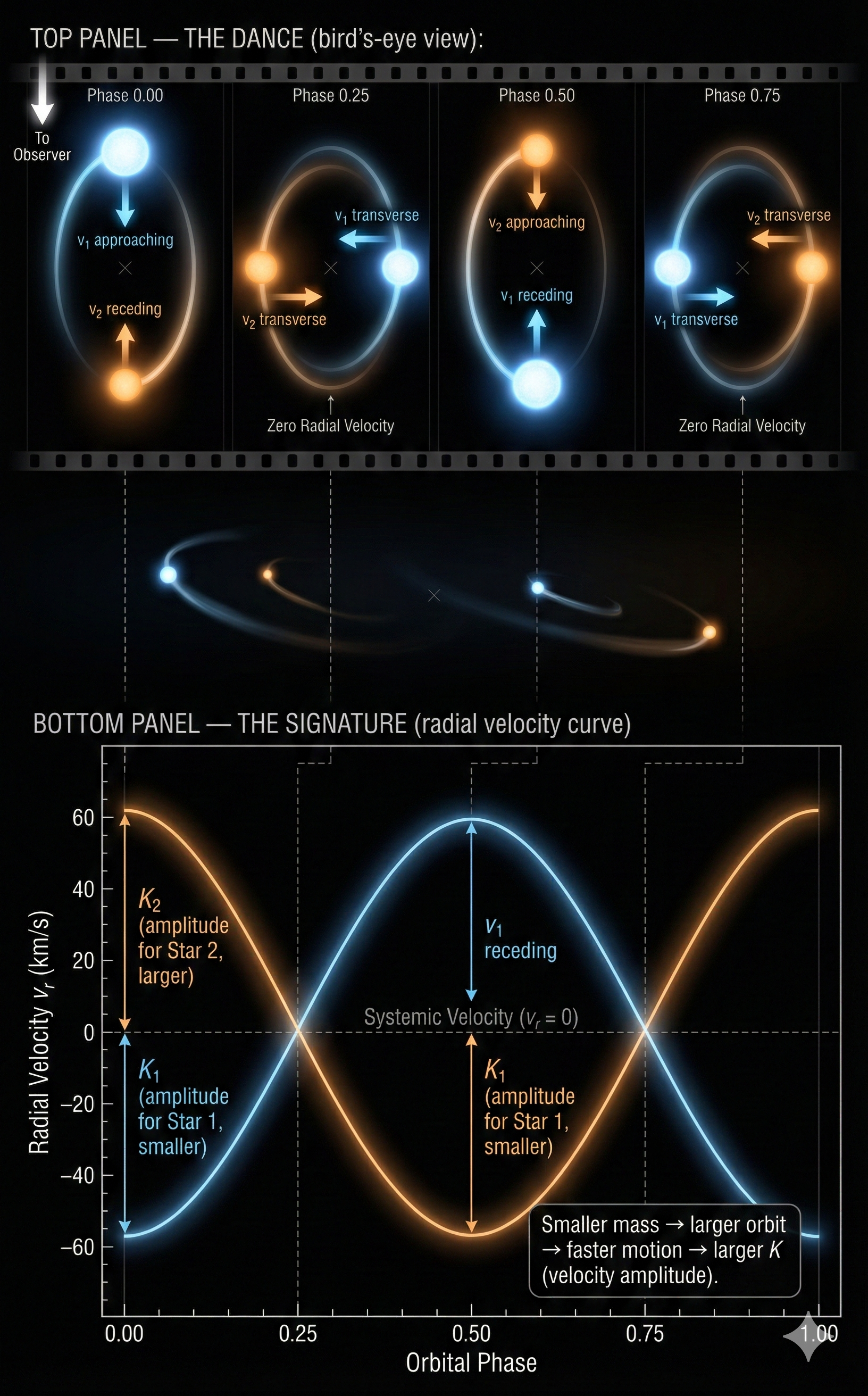
A star in a binary orbits the center of mass: during half the orbit it moves toward us, during the other half away. Its spectral lines shift back and forth — blueshifted approaching, redshifted receding — with a period equal to the orbital period. A spectroscopic binary is detected by this periodic Doppler wobble. Lecture 3 already showed a preview: the worked example of a star with Hα oscillating between $656.25\,\text{nm}$ and $656.35\,\text{nm}$ over $4.0\,\text{days}$ — that was a spectroscopic binary.

Spectroscopic binary

A binary detected from the periodic Doppler oscillation of its spectral lines as the stars orbit. It yields the period $P$ and radial-velocity amplitude $K$ even when the pair is far too close to resolve.

What spectroscopic binaries give us:

Orbital period $P$ (from the Doppler oscillation)
Radial-velocity amplitude $K$ (half the peak-to-peak velocity swing) — directly from the Doppler shift
If both stars’ lines are visible (a double-lined binary, SB2), we get $K_1$ and $K_2$ separately

Key connection to Lecture 3: the Doppler formula $\Delta\lambda/\lambda_0 = v_r/c$ converts wavelength shifts to velocities. Now we use those velocities as a function of time to trace the orbit.

Eclipsing Binaries: Light Curves Reveal Geometry

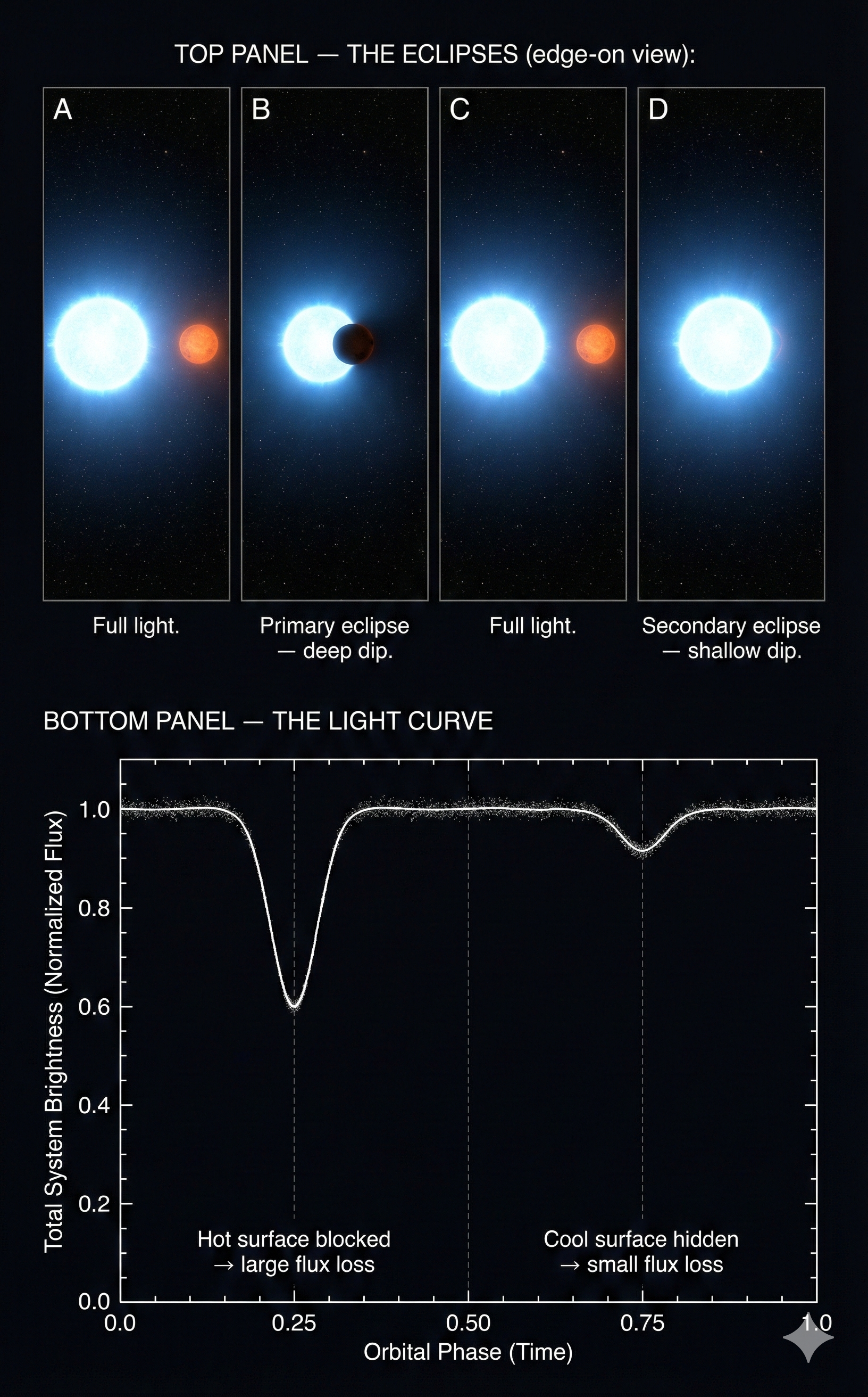
When the orbital plane is nearly edge-on, the stars periodically pass in front of each other. These are eclipsing binaries, and they produce characteristic dips in the combined light — a light curve.

Eclipsing binary

A binary whose orbit is nearly edge-on, so the stars periodically eclipse each other. The eclipses pin the inclination near $90^\circ$ and reveal the relative stellar radii and temperature ratio.

Light curve

A plot of a source’s brightness versus time. For an eclipsing binary, the spacing, depth, and shape of its dips encode the period, radii, and temperature ratio.

What eclipsing binaries give us:

Orbital period $P$ (from the spacing between eclipses)
Relative stellar radii (from the duration and shape of eclipses)
Inclination $i \approx 90^\circ$ (the orbit must be nearly edge-on for eclipses)
Temperature ratio (from the relative depths of primary and secondary eclipses)

The inclination is the prize: it removes the biggest uncertainty in spectroscopic measurements (below). The gold standard: a system that is both eclipsing and double-lined spectroscopic gives everything — period, both velocity amplitudes, inclination, and both radii — for the most precise stellar masses available (uncertainties of 1%–2%).

Classic example: Algol (β Persei), one of the first-known eclipsing binaries, dips every $2.87\,\text{days}$ as its cooler companion crosses the hot primary.

Summary: What Each Type Reveals

Binary Type	How Detected	What It Gives	What It Misses
Visual	Resolved on sky	$P$ , $a$ (with distance), mass ratio	Needs decades; nearby only
Spectroscopic	Doppler wobble	$P$ , $K_1$ (and $K_2$ if SB2)	Inclination $i$ unknown (only $v\sin i$ )
Eclipsing	Light-curve dips	$P$ , $i \approx 90^\circ$ , relative radii, $T$ ratio	Rare edge-on geometry
Eclipsing + SB2	Both	Everything: $M_1$ , $M_2$ , $R_1$ , $R_2$ , $T_1/T_2$	Rarest; edge-on and bright enough

Problem

Why can’t you measure a star’s mass from its spectrum alone?
A binary has period $30\,\text{yr}$ and the stars are resolved in a telescope. What type is it?
You observe a star whose Hα line oscillates between $656.2\,\text{nm}$ and $656.4\,\text{nm}$ every $10\,\text{days}$ . What type is it, and what can you immediately determine?

Quick check

Your lab partner says: “A star whose lines shift periodically and whose brightness dips periodically — that’s the jackpot.” Explain why this combination is so powerful. What specific problem does the eclipsing geometry solve that spectroscopy alone cannot?

Why this has to work. We need only two physics ingredients: Newtonian two-body gravity and the center-of-mass condition linking the stars. On the observation side: time variation (for $P$ ), line-of-sight velocities (for $K_1$ , $K_2$ ), and geometry (inclination $i$ ). That structure forces a specific chain: $P \to a$ ; velocity-amplitude ratio $\to$ mass ratio; total mass + mass ratio $\to$ individual masses. Once measured, there is no alternative dynamical route to $M_1$ and $M_2$ .

Extracting Masses from Orbits

Part 3: Extracting Masses from Orbits

We have the observational tools. How do we go from measured quantities ( $P$ , $K_1$ , $K_2$ ) to masses ( $M_1$ , $M_2$ )? The physics is entirely from Module 1 — Kepler’s third law and Newton’s third law — applied to a two-body system.

Multiple choice

Two stars orbit their common center of mass with $K_1=80$ km/s and $K_2=200$ km/s. Which star is more massive, and which has the larger orbit?

Star 1 (smaller K) is more massive; Star 2 has the larger orbitStar 2 (larger K) is more massive; Star 2 has the larger orbitStar 1 is more massive; Star 1 has the larger orbit

Step 1: Newton’s Kepler III for Binaries

In Module 1 you derived Newton’s version of Kepler’s third law for a planet orbiting a star — and the key insight was that the mass of the central body appears: $P^2 = 4\pi^2 r^3 / GM$ . But that assumed the planet’s mass was negligible ( $m \ll M$ ). In a binary, both masses matter. Newton’s full two-body form is the mass-bearing relation:

Here $P$ is the orbital period, $a = a_1 + a_2$ is the total separation (the semi-major axis of the relative orbit), $M_1, M_2$ are the masses, and $G = 6.67 \times 10^{-8}\,\text{cm}^3\,\text{g}^{-1}\,\text{s}^{-2}$ . Two things changed from the planetary case: $M$ became $M_1 + M_2$ , and $r$ became $a$ .

Rearranging gives the total mass $M_1 + M_2 = 4\pi^2 a^3 / G P^2$ . If we measure $P$ and $a$ , we get the total mass — but we still need to separate $M_1$ from $M_2$ .

Step 2: The Center-of-Mass Condition

Both stars orbit the center of mass — the balance point. Newton’s third law guarantees it: if star 1 pulls on star 2 with force $F$ , star 2 pulls back with $F$ . Both accelerate, but the more massive star has the smaller orbit.

Center of mass

The balance point of a system, about which both stars orbit. For a binary it lies on the line joining the stars, always closer to the heavier one, fixed by $M_1 a_1 = M_2 a_2$ .

Mass ratio

The ratio $M_1/M_2$ of the two stellar masses — equal to the inverse ratio of their orbital sizes ( $a_2/a_1$ ) and to the ratio of their velocity amplitudes ( $K_2/K_1$ ), independent of inclination.

Diagram titled Binary Star Orbits and Center of Mass on black background. A large yellow-white star labeled M₁ on the left and a smaller orange star labeled M₂ on the right are connected through a white × labeled CM (center of mass), positioned closer to M₁. Dashed elliptical orbits show M₁ tracing a small orbit of radius a₁ and M₂ tracing a large orbit of radius a₂, both centered on the CM. A bracket below spans the full separation labeled a = a₁ + a₂. Epoch dots along each orbit show the stars always on opposite sides. Text reads: Stars move in synchronous elliptical orbits, always on opposite sides of the CM. — Figure 6The center of mass is the pivot point — always closer to the heavier star. M1 barely moves (a1 small); M2 swings wide (a2 large). The balance condition M1 a1 = M2 a2 means the mass ratio equals the inverse ratio of orbital sizes. Epoch dots show the stars always on opposite sides of the CM.ASTR 201 (Gemini)

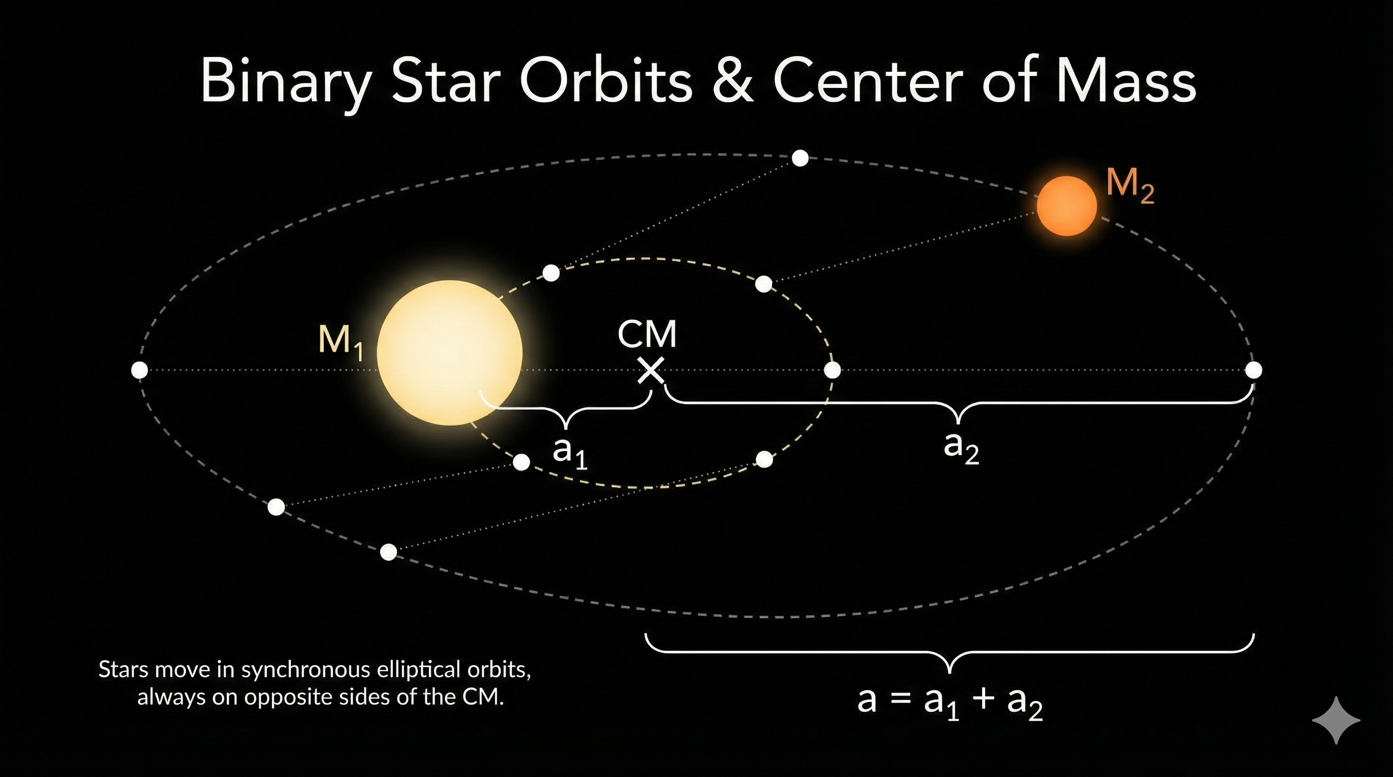
The center-of-mass condition is:

so $M_1/M_2 = a_2/a_1$ . The mass ratio is the inverse of the orbit-size ratio: the heavier star barely moves while the lighter swings wide.

Step 3: Connecting Velocities to Orbits

For spectroscopic binaries we measure velocities, not $a_1$ and $a_2$ . For circular orbits, $v_1 = 2\pi a_1/P$ and $v_2 = 2\pi a_2/P$ . Since the period is shared, the velocity ratio equals the orbit-size ratio:

$\frac{v_1}{v_2} = \frac{a_1}{a_2} = \frac{M_2}{M_1}$

In practice we measure the radial-velocity amplitudes $K_1, K_2$ — the maximum line-of-sight velocities. For an orbit with inclination $i$ (where $i = 90^\circ$ is edge-on, $i = 0^\circ$ face-on), $K_1 = v_1 \sin i$ and $K_2 = v_2 \sin i$ . The ratio is inclination-independent (the $\sin i$ cancels):

$\frac{M_1}{M_2} = \frac{K_2}{K_1}$

The mass ratio comes directly from the velocity ratio, regardless of inclination.

Step 4: Putting It All Together

For an SB2 — where we measure $P$ , $K_1$ , $K_2$ — we determine both masses if we know $i$ . From velocities and period, the projected orbital radii are $a_1 \sin i = K_1 P / 2\pi$ and $a_2 \sin i = K_2 P / 2\pi$ , so the projected total separation is $a \sin i = (K_1 + K_2)P/2\pi$ . Substituting into Kepler III:

$M_1 + M_2 = \frac{4\pi^2 (a\sin i)^3}{G\,P^2 \sin^3 i} = \frac{(K_1 + K_2)^3\, P}{2\pi\, G\, \sin^3 i}$

Combined with $M_1/M_2 = K_2/K_1$ , we solve for each mass individually. The measured Doppler amplitude is a projected speed, $K = v\sin i$ , so each velocity carries one factor of $\sin i$ ; that propagates into the orbital scale as $a\sin i$ , and because Kepler depends on the cube of separation, it appears as a cubic correction $\sin^3 i$ in the inferred mass.

Inclination

The tilt angle $i$ of an orbital plane relative to the plane of the sky: $i = 90^\circ$ is edge-on (eclipses possible, full radial velocity) and $i = 0^\circ$ is face-on (no Doppler signal). It enters binary masses as a $\sin^3 i$ factor.

Worked Example 1Weighing a Spectroscopic Binary

Problem

An eclipsing, double-lined spectroscopic binary has $P = 3.00\,\text{days} = 2.59 \times 10^5\,\text{s}$ , $K_1 = 80\,\text{km/s} = 8.0 \times 10^6\,\text{cm/s}$ , $K_2 = 200\,\text{km/s} = 2.0 \times 10^7\,\text{cm/s}$ , and $i = 90^\circ$ ( $\sin i = 1$ ). Find $M_1$ and $M_2$ .

StepMass ratio from velocity ratio

$\frac{M_1}{M_2} = \frac{K_2}{K_1} = \frac{200}{80} = 2.5$ Star 1 is 2.5 times more massive — the heavier star moves slower, closer to the center of mass.

StepTotal separation from velocities and period

$a = \frac{(K_1 + K_2)P}{2\pi} = \frac{(2.8 \times 10^7\,\text{cm/s})(2.59 \times 10^5\,\text{s})}{6.28} = 1.15 \times 10^{12}\,\text{cm}$ For reference $1\,\text{AU} = 1.50 \times 10^{13}\,\text{cm}$ , so $a \approx 0.077\,\text{AU}$ — a tight orbit.

StepTotal mass from Kepler's third law

$M_1 + M_2 = \frac{4\pi^2 a^3}{G P^2} = \frac{6.01 \times 10^{37}\,\text{cm}^3}{4.47 \times 10^{3}\,\text{cm}^3\,\text{g}^{-1}} = 1.34 \times 10^{34}\,\text{g} = 6.7\,M_\odot$ (using $M_\odot = 1.99 \times 10^{33}\,\text{g}$ ).

StepIndividual masses from the ratio

$M_2 = \frac{6.7\,M_\odot}{1 + 2.5} = 1.9\,M_\odot \qquad M_1 = 2.5 \times 1.9\,M_\odot = 4.8\,M_\odot$

Dimensional check

Started with cm, s, and $G$ in CGS → grams → converted to $M_\odot$ . The numerator $4\pi^2 a^3$ is $\text{cm}^3$ ; the denominator $GP^2$ is $\text{cm}^3\,\text{g}^{-1}$ ; the quotient is grams ✓.

Result

Star 1 ( $K_1 = 80\,\text{km/s}$ ) moves slower → heavier → $4.8\,M_\odot$ . Star 2 ( $K_2 = 200\,\text{km/s}$ ) moves faster → lighter → $1.9\,M_\odot$ . A $4.8\,M_\odot$ star is a late B-type star, consistent with being the brighter component ✓.

The Scaling Approach: Using Solar Units

The worked example used full CGS arithmetic — instructive but laborious. In practice, astronomers use a scaling version of Kepler III that avoids large numbers. For the Sun-Earth system ( $P = 1\,\text{yr}$ , $a = 1\,\text{AU}$ , $M_\odot + M_\oplus \approx M_\odot$ ), dividing the binary equation by the solar one gives the solar-unit working form shown on the kepler-binary card above:

$\left(\frac{P}{1\,\text{yr}}\right)^2 = \frac{(a/\text{AU})^3}{(M_1 + M_2)/M_\odot} \quad\Longleftrightarrow\quad \frac{M_1 + M_2}{M_\odot} = \frac{(a/\text{AU})^3}{(P/\text{yr})^2}$

All the constants ( $4\pi^2$ , $G$ ) are absorbed into the units. Measure $a$ in AU and $P$ in years, and you get total mass in solar masses — no calculator needed for order-of-magnitude work.

Problem

A visual binary has $P = 50\,\text{yr}$ and $a = 20\,\text{AU}$ . What is the total mass?
Two equal-mass stars orbit with $P = 1\,\text{yr}$ at $a = 1\,\text{AU}$ . What is each star’s mass?
If you double the separation at fixed total mass, by what factor does the period increase?

Deep Dive: Enrichment: The Mass Function (SB1 Systems)

What if only one star’s lines are visible — a single-lined spectroscopic binary (SB1)? You measure $P$ and $K_1$ but not $K_2$ . You can still learn something, via the mass function:

$f(M_2) = \frac{M_2^3 \sin^3 i}{(M_1 + M_2)^2} = \frac{K_1^3\, P}{2\pi\, G}$

The right side is entirely measured; the left contains three unknowns ( $M_1$ , $M_2$ , $i$ ). So the mass function is a lower limit on $M_2$ (since $\sin i \leq 1$ ). With an independent estimate of $M_1$ (e.g. from spectral type), you constrain $M_2$ more tightly. This is how astronomers found some of the first stellar-mass black holes — the unseen companion was too massive to be a neutron star.

Over more than a century, these techniques — visual, spectroscopic, eclipsing, and combinations — have been applied to hundreds of systems, with the tightest constraints from eclipsing SB2 binaries. The dynamical problem is solved: mass is no longer hidden if the orbit is well measured. That flips the question. Instead of asking how to measure mass, we can ask what mass controls.

The Mass–Luminosity Relation and Synthesis

Part 4: The Mass-Luminosity Relation — The Empirical Payoff

Multiple choice

The Sun ( $1\,M_\odot$ ) has $L=1\,L_\odot$ . A main-sequence star with twice the Sun’s mass is how much more luminous?

About 2× (linear in mass)About 4× (mass squared)Much larger — about 10× or more

Building the Relation from Data

Astronomers have spent over a century measuring binary-star masses. For each system with individual masses, the luminosity is also measured (from apparent brightness and distance). You might expect a mess — stars differ in composition, age, rotation, evolutionary state. But when you plot mass against luminosity, both in solar units, both logarithmic, the expected scatter simply isn’t there.

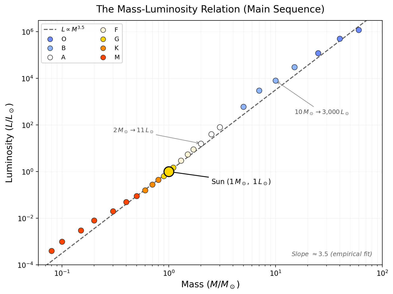
Log-log plot of luminosity versus mass for main-sequence stars in solar units. Points are color-coded by spectral type (blue for O/B, white for A, yellow for G, orange for K, red for M). A dashed line shows the power-law fit L proportional to M to the 3.5. The Sun is marked at (1, 1). Annotations show that 2 solar masses gives about 11 solar luminosities and 10 solar masses gives about 3000 solar luminosities. — Figure 7Main-sequence stars follow a tight power law L proportional to M^3.5 — a modest increase in mass produces a dramatic increase in luminosity. The Sun sits in the middle. Built entirely from binary star mass measurements, this relation proves mass is the master variable.ASTR 201 (generated)

The idealized power law captures the trend; real data have scatter:

Log-log scatter plot of stellar luminosity in solar units versus mass in solar units from Eker et al. 2018. Hundreds of gray data points form a tight diagonal band from lower-left (low mass, low luminosity) to upper-right (high mass, high luminosity). A red piecewise linear fit and blue dotted classical power-law fit overlay the data. Short vertical tick marks along the horizontal axis indicate mass boundaries between the four power-law segments. — Figure 8Real mass-luminosity data from 509 binary star components with dynamically measured masses. The red line is a piecewise four-segment power-law fit; the blue dotted line is the classical single power law. The relation steepens at high masses (L proportional to M^~4) and flattens at low masses (L proportional to M^~2.3). Scatter increases above ~3 solar masses where stellar evolution is faster.Eker et al. 2018, MNRAS 479, 5491

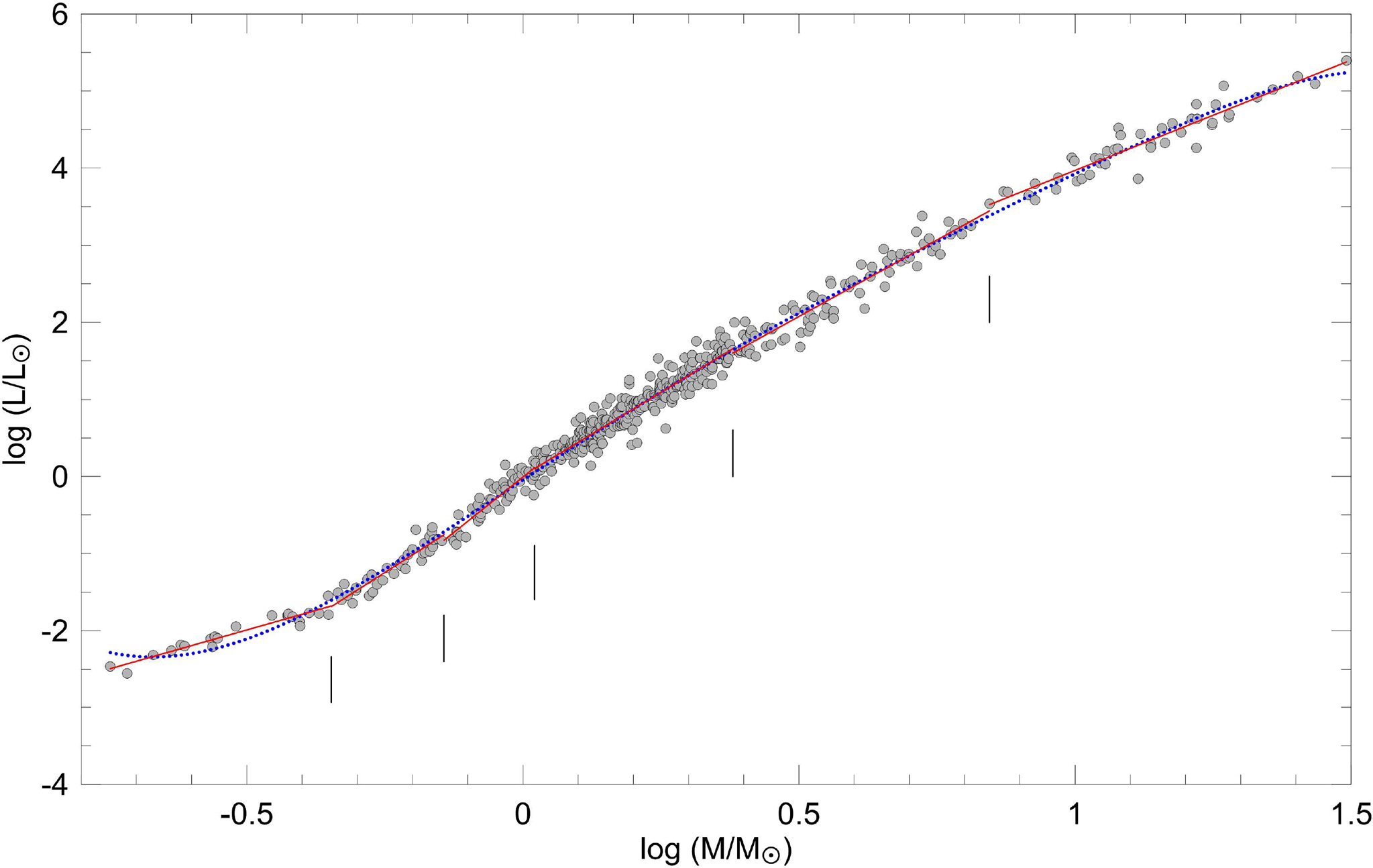
Main-sequence stars fall on a tight power law — the mass-luminosity relation:

The exponent is the lever arm: a small shift in mass produces a disproportionate shift in luminosity, so the main sequence is a mass sequence in disguise. In Module 3, the same leverage reappears in evolution — timescales and stellar endpoints trace back to how sharply luminosity responds to mass.

Mass-luminosity relation

The empirical scaling $L/L_\odot \approx (M/M_\odot)^{3.5}$ for main-sequence stars, calibrated entirely from binary-star masses. The steep exponent makes mass the master variable that predicts luminosity, lifetime, and fate.

The exponent $3.5$ is an approximation — slightly steeper at high masses (about $4$ above $2\,M_\odot$ ) and shallower at low masses (about $2.3$ below $0.43\,M_\odot$ ) — but it captures the essential behavior across a wide range.

What the Relation Tells Us

A modest change in mass produces a dramatic change in luminosity:

Mass ( $M_\odot$ )	$L/L_\odot \approx (M/M_\odot)^{3.5}$	Factor vs. Sun
$0.1$	$3.2 \times 10^{-4}$	$3 \times 10^3$ fainter
$0.5$	$0.088$	$11$ fainter
$1.0$	$1.0$	the Sun
$2.0$	$11.3$	$11$ brighter
$10$	$3.16 \times 10^3$	$\sim 3 \times 10^3$ brighter
$50$	$8.8 \times 10^5$	$\sim 10^6$ brighter

The full range of main-sequence masses (about $0.08\,M_\odot$ to $150\,M_\odot$ ) spans roughly three orders of magnitude in mass — but the luminosity range spans ten orders of magnitude.

Why Mass Controls Lifetime

Once luminosity scales this steeply, lifetime becomes an exponent game. A star’s fuel scales with its mass $M$ ; its luminosity — the burn rate — scales as $M^{3.5}$ , so $t_{\text{MS}} \propto M/L \propto M^{-2.5}$ .

More massive stars live much shorter lives. The Sun’s main-sequence lifetime is about $10\,\text{Gyr}$ . A $10\,M_\odot$ star lives $\sim 30\,\text{Myr}$ — roughly 300 times shorter. A $0.5\,M_\odot$ star lives $\sim 57\,\text{Gyr}$ . Pause on that: the universe is $13.8\,\text{Gyr}$ old, so a $0.5\,M_\odot$ red dwarf born at the Big Bang is not even a quarter through its main-sequence life. Every low-mass star that has ever formed is still shining today. The graveyard of stellar evolution holds only the remains of massive stars — the ones that burned bright and fast.

Problem

Estimate the luminosity of a $5\,M_\odot$ main-sequence star.
Estimate its main-sequence lifetime (Sun’s is $\sim 10\,\text{Gyr}$ ).
Two main-sequence stars have $L_A = 100\,L_\odot$ and $L_B = 0.01\,L_\odot$ . Estimate the ratio of their masses.
Why does the mass-luminosity relation apply only to main-sequence stars?

Observable → Model → Inference: The Binary Star Chain

Observable

Periodic shifts in spectral-line wavelengths (and brightness dips, if eclipsing)

A star’s lines oscillate blueshift-to-redshift over the orbital period; in eclipsing systems the combined light dips on the same cycle. Both are time-domain measurements.

Model

Two stars orbiting a common center of mass under Newtonian gravity

Kepler’s third law connects the orbit to the total mass; the center-of-mass condition (Newton’s third law) connects the velocity amplitudes to the mass ratio.

Inference

Individual stellar masses — and, across many systems, the mass-luminosity relation

From $P$ , $K_1$ , $K_2$ , $i$ we get $M_1$ and $M_2$ ; from a large sample, $L \propto M^{3.5}$ , the most important empirical scaling in stellar astrophysics.

The inference runs as a cascade: the measured quantities ( $P$ , $K_1$ , $K_2$ , and $i$ if eclipsing, or $a$ if visual with distance) feed the two-body model, which yields the orbital scale ( $a$ or $a\sin i$ ), then the dynamical outputs ( $M_{\text{total}}$ and $M_1/M_2$ ), then the individual masses ( $M_1$ , $M_2$ ) — and finally the downstream physics: $L \propto M^{3.5} \to t_{\text{MS}} \propto M^{-2.5} \to$ stellar fate.

Connection: The Module 2 Inference Chain — Complete

Each lecture in Module 2 added one link. The chain is now complete:

Lecture	Tool	Question	What It Unlocks
1	Parallax → distance	How far?	Distance $d$ ; then $L = 4\pi d^2 F$
2	Color/flux → temperature; Stefan-Boltzmann	How hot? How big?	Temperature $T$ ; radius $R$
3	Spectral lines → composition, Doppler	Made of? Moving how?	Composition; radial velocity
4	Binary orbits → mass	How heavy?	Mass $M$ ; mass-luminosity relation

Combined: from photons alone we can now characterize every fundamental stellar property — distance, luminosity, temperature, radius, composition, and mass. Next: we put everything on one diagram — the HR diagram — and the patterns it reveals demand a physical explanation.

Summary: The Last Piece

Mass is the master variable — it determines luminosity, temperature, radius, lifetime, and death. But it can’t be measured from a single star’s light.
Binary stars reveal masses through orbital dynamics — visual binaries give orbits on the sky, spectroscopic binaries give Doppler velocities, eclipsing binaries give inclination and radii.
Newton’s Kepler III for binaries ( $P^2 = 4\pi^2 a^3 / G(M_1 + M_2)$ ) gives the total mass; the center-of-mass condition ( $M_1 a_1 = M_2 a_2$ ) gives the mass ratio from the velocity ratio.
The mass-luminosity relation ( $L \propto M^{3.5}$ ) is the most important empirical scaling in stellar astrophysics — a factor of 10 in mass produces $\sim 3 \times 10^3$ in luminosity.
Lifetime scales as $M^{-2.5}$ — massive stars burn bright and die young; low-mass stars are dim but nearly eternal.

Glossary

Center of mass: The balance point of a system, about which both stars orbit. For a binary it lies on the line joining the stars, always closer to the heavier one, fixed by $M_1 a_1 = M_2 a_2$ .
Eclipsing binary: A binary whose orbit is nearly edge-on, so the stars periodically eclipse each other. The eclipses pin the inclination near $90^\circ$ and reveal the relative stellar radii and temperature ratio.
Inclination: The tilt angle $i$ of an orbital plane relative to the plane of the sky: $i = 90^\circ$ is edge-on (eclipses possible, full radial velocity) and $i = 0^\circ$ is face-on (no Doppler signal). It enters binary masses as a $\sin^3 i$ factor.
Light curve: A plot of a source’s brightness versus time. For an eclipsing binary, the spacing, depth, and shape of its dips encode the period, radii, and temperature ratio.
Main sequence: The band on the H–R diagram where stars spend most of their lives in stable hydrogen-core fusion. A main-sequence star’s position is set almost entirely by its mass.
Mass ratio: The ratio $M_1/M_2$ of the two stellar masses — equal to the inverse ratio of their orbital sizes ( $a_2/a_1$ ) and to the ratio of their velocity amplitudes ( $K_2/K_1$ ), independent of inclination.
Mass-luminosity relation: The empirical scaling $L/L_\odot \approx (M/M_\odot)^{3.5}$ for main-sequence stars, calibrated entirely from binary-star masses. The steep exponent makes mass the master variable that predicts luminosity, lifetime, and fate.
Spectroscopic binary: A binary detected from the periodic Doppler oscillation of its spectral lines as the stars orbit. It yields the period $P$ and radial-velocity amplitude $K$ even when the pair is far too close to resolve.
Visual binary: A binary whose two stars are individually resolved through a telescope, so their orbits can be traced directly on the sky over years to decades.
White dwarf: The dense, Earth-sized remnant left when a low- or intermediate-mass star exhausts its fuel — about a solar mass packed into a planetary volume, shining only from stored heat.