Weighing Stars

Section 3 of 4

Extracting Masses from Orbits

Part 3: Extracting Masses from Orbits

We have the observational tools. How do we go from measured quantities ( $P$ , $K_1$ , $K_2$ ) to masses ( $M_1$ , $M_2$ )? The physics is entirely from Module 1 — Kepler’s third law and Newton’s third law — applied to a two-body system.

Multiple choice

Two stars orbit their common center of mass with $K_1=80$ km/s and $K_2=200$ km/s. Which star is more massive, and which has the larger orbit?

Star 1 (smaller K) is more massive; Star 2 has the larger orbitStar 2 (larger K) is more massive; Star 2 has the larger orbitStar 1 is more massive; Star 1 has the larger orbit

Step 1: Newton’s Kepler III for Binaries

In Module 1 you derived Newton’s version of Kepler’s third law for a planet orbiting a star — and the key insight was that the mass of the central body appears: $P^2 = 4\pi^2 r^3 / GM$ . But that assumed the planet’s mass was negligible ( $m \ll M$ ). In a binary, both masses matter. Newton’s full two-body form is the mass-bearing relation:

Here $P$ is the orbital period, $a = a_1 + a_2$ is the total separation (the semi-major axis of the relative orbit), $M_1, M_2$ are the masses, and $G = 6.67 \times 10^{-8}\,\text{cm}^3\,\text{g}^{-1}\,\text{s}^{-2}$ . Two things changed from the planetary case: $M$ became $M_1 + M_2$ , and $r$ became $a$ .

Rearranging gives the total mass $M_1 + M_2 = 4\pi^2 a^3 / G P^2$ . If we measure $P$ and $a$ , we get the total mass — but we still need to separate $M_1$ from $M_2$ .

Step 2: The Center-of-Mass Condition

Both stars orbit the center of mass — the balance point. Newton’s third law guarantees it: if star 1 pulls on star 2 with force $F$ , star 2 pulls back with $F$ . Both accelerate, but the more massive star has the smaller orbit.

Center of mass

The balance point of a system, about which both stars orbit. For a binary it lies on the line joining the stars, always closer to the heavier one, fixed by $M_1 a_1 = M_2 a_2$ .

Mass ratio

The ratio $M_1/M_2$ of the two stellar masses — equal to the inverse ratio of their orbital sizes ( $a_2/a_1$ ) and to the ratio of their velocity amplitudes ( $K_2/K_1$ ), independent of inclination.

Diagram titled Binary Star Orbits and Center of Mass on black background. A large yellow-white star labeled M₁ on the left and a smaller orange star labeled M₂ on the right are connected through a white × labeled CM (center of mass), positioned closer to M₁. Dashed elliptical orbits show M₁ tracing a small orbit of radius a₁ and M₂ tracing a large orbit of radius a₂, both centered on the CM. A bracket below spans the full separation labeled a = a₁ + a₂. Epoch dots along each orbit show the stars always on opposite sides. Text reads: Stars move in synchronous elliptical orbits, always on opposite sides of the CM. — Figure 6The center of mass is the pivot point — always closer to the heavier star. M1 barely moves (a1 small); M2 swings wide (a2 large). The balance condition M1 a1 = M2 a2 means the mass ratio equals the inverse ratio of orbital sizes. Epoch dots show the stars always on opposite sides of the CM.ASTR 201 (Gemini)

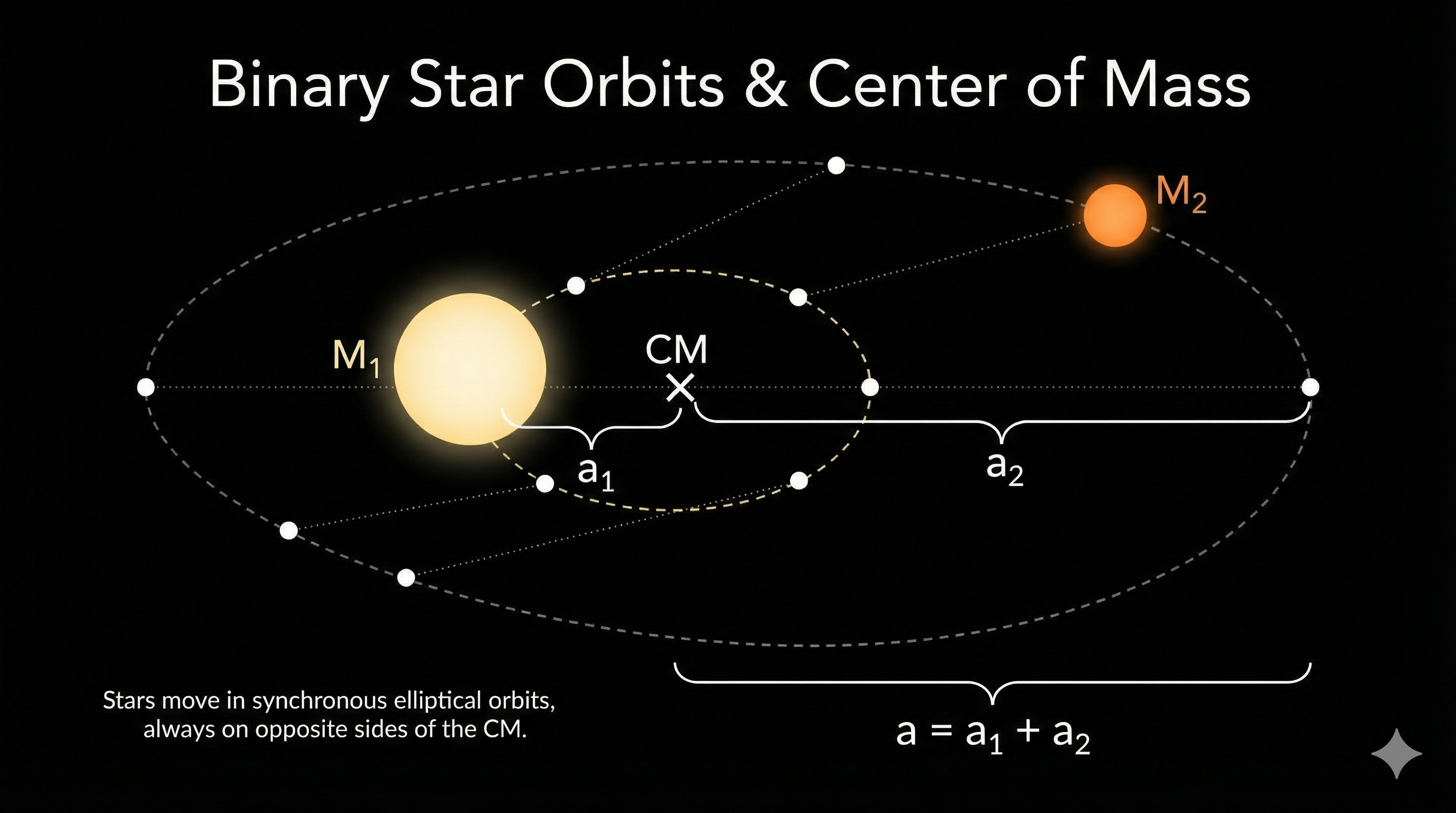
The center-of-mass condition is:

so $M_1/M_2 = a_2/a_1$ . The mass ratio is the inverse of the orbit-size ratio: the heavier star barely moves while the lighter swings wide.

Step 3: Connecting Velocities to Orbits

For spectroscopic binaries we measure velocities, not $a_1$ and $a_2$ . For circular orbits, $v_1 = 2\pi a_1/P$ and $v_2 = 2\pi a_2/P$ . Since the period is shared, the velocity ratio equals the orbit-size ratio:

$\frac{v_1}{v_2} = \frac{a_1}{a_2} = \frac{M_2}{M_1}$

In practice we measure the radial-velocity amplitudes $K_1, K_2$ — the maximum line-of-sight velocities. For an orbit with inclination $i$ (where $i = 90^\circ$ is edge-on, $i = 0^\circ$ face-on), $K_1 = v_1 \sin i$ and $K_2 = v_2 \sin i$ . The ratio is inclination-independent (the $\sin i$ cancels):

$\frac{M_1}{M_2} = \frac{K_2}{K_1}$

The mass ratio comes directly from the velocity ratio, regardless of inclination.

Step 4: Putting It All Together

For an SB2 — where we measure $P$ , $K_1$ , $K_2$ — we determine both masses if we know $i$ . From velocities and period, the projected orbital radii are $a_1 \sin i = K_1 P / 2\pi$ and $a_2 \sin i = K_2 P / 2\pi$ , so the projected total separation is $a \sin i = (K_1 + K_2)P/2\pi$ . Substituting into Kepler III:

$M_1 + M_2 = \frac{4\pi^2 (a\sin i)^3}{G\,P^2 \sin^3 i} = \frac{(K_1 + K_2)^3\, P}{2\pi\, G\, \sin^3 i}$

Combined with $M_1/M_2 = K_2/K_1$ , we solve for each mass individually. The measured Doppler amplitude is a projected speed, $K = v\sin i$ , so each velocity carries one factor of $\sin i$ ; that propagates into the orbital scale as $a\sin i$ , and because Kepler depends on the cube of separation, it appears as a cubic correction $\sin^3 i$ in the inferred mass.

Inclination

The tilt angle $i$ of an orbital plane relative to the plane of the sky: $i = 90^\circ$ is edge-on (eclipses possible, full radial velocity) and $i = 0^\circ$ is face-on (no Doppler signal). It enters binary masses as a $\sin^3 i$ factor.

Worked Example 1Weighing a Spectroscopic Binary

Problem

An eclipsing, double-lined spectroscopic binary has $P = 3.00\,\text{days} = 2.59 \times 10^5\,\text{s}$ , $K_1 = 80\,\text{km/s} = 8.0 \times 10^6\,\text{cm/s}$ , $K_2 = 200\,\text{km/s} = 2.0 \times 10^7\,\text{cm/s}$ , and $i = 90^\circ$ ( $\sin i = 1$ ). Find $M_1$ and $M_2$ .

StepMass ratio from velocity ratio

$\frac{M_1}{M_2} = \frac{K_2}{K_1} = \frac{200}{80} = 2.5$ Star 1 is 2.5 times more massive — the heavier star moves slower, closer to the center of mass.

StepTotal separation from velocities and period

$a = \frac{(K_1 + K_2)P}{2\pi} = \frac{(2.8 \times 10^7\,\text{cm/s})(2.59 \times 10^5\,\text{s})}{6.28} = 1.15 \times 10^{12}\,\text{cm}$ For reference $1\,\text{AU} = 1.50 \times 10^{13}\,\text{cm}$ , so $a \approx 0.077\,\text{AU}$ — a tight orbit.

StepTotal mass from Kepler's third law

$M_1 + M_2 = \frac{4\pi^2 a^3}{G P^2} = \frac{6.01 \times 10^{37}\,\text{cm}^3}{4.47 \times 10^{3}\,\text{cm}^3\,\text{g}^{-1}} = 1.34 \times 10^{34}\,\text{g} = 6.7\,M_\odot$ (using $M_\odot = 1.99 \times 10^{33}\,\text{g}$ ).

StepIndividual masses from the ratio

$M_2 = \frac{6.7\,M_\odot}{1 + 2.5} = 1.9\,M_\odot \qquad M_1 = 2.5 \times 1.9\,M_\odot = 4.8\,M_\odot$

Dimensional check

Started with cm, s, and $G$ in CGS → grams → converted to $M_\odot$ . The numerator $4\pi^2 a^3$ is $\text{cm}^3$ ; the denominator $GP^2$ is $\text{cm}^3\,\text{g}^{-1}$ ; the quotient is grams ✓.

Result

Star 1 ( $K_1 = 80\,\text{km/s}$ ) moves slower → heavier → $4.8\,M_\odot$ . Star 2 ( $K_2 = 200\,\text{km/s}$ ) moves faster → lighter → $1.9\,M_\odot$ . A $4.8\,M_\odot$ star is a late B-type star, consistent with being the brighter component ✓.

The Scaling Approach: Using Solar Units

The worked example used full CGS arithmetic — instructive but laborious. In practice, astronomers use a scaling version of Kepler III that avoids large numbers. For the Sun-Earth system ( $P = 1\,\text{yr}$ , $a = 1\,\text{AU}$ , $M_\odot + M_\oplus \approx M_\odot$ ), dividing the binary equation by the solar one gives the solar-unit working form shown on the kepler-binary card above:

$\left(\frac{P}{1\,\text{yr}}\right)^2 = \frac{(a/\text{AU})^3}{(M_1 + M_2)/M_\odot} \quad\Longleftrightarrow\quad \frac{M_1 + M_2}{M_\odot} = \frac{(a/\text{AU})^3}{(P/\text{yr})^2}$

All the constants ( $4\pi^2$ , $G$ ) are absorbed into the units. Measure $a$ in AU and $P$ in years, and you get total mass in solar masses — no calculator needed for order-of-magnitude work.

Problem

A visual binary has $P = 50\,\text{yr}$ and $a = 20\,\text{AU}$ . What is the total mass?
Two equal-mass stars orbit with $P = 1\,\text{yr}$ at $a = 1\,\text{AU}$ . What is each star’s mass?
If you double the separation at fixed total mass, by what factor does the period increase?

Deep Dive: Enrichment: The Mass Function (SB1 Systems)

What if only one star’s lines are visible — a single-lined spectroscopic binary (SB1)? You measure $P$ and $K_1$ but not $K_2$ . You can still learn something, via the mass function:

$f(M_2) = \frac{M_2^3 \sin^3 i}{(M_1 + M_2)^2} = \frac{K_1^3\, P}{2\pi\, G}$

The right side is entirely measured; the left contains three unknowns ( $M_1$ , $M_2$ , $i$ ). So the mass function is a lower limit on $M_2$ (since $\sin i \leq 1$ ). With an independent estimate of $M_1$ (e.g. from spectral type), you constrain $M_2$ more tightly. This is how astronomers found some of the first stellar-mass black holes — the unseen companion was too massive to be a neutron star.

Over more than a century, these techniques — visual, spectroscopic, eclipsing, and combinations — have been applied to hundreds of systems, with the tightest constraints from eclipsing SB2 binaries. The dynamical problem is solved: mass is no longer hidden if the orbit is well measured. That flips the question. Instead of asking how to measure mass, we can ask what mass controls.