Lecture 1: Distance & Parallax

How far? The foundation of stellar astrophysics

Measuring distance is the fundamental problem in astronomy. This lecture introduces parallax, derives the inverse-square law, and shows how distance unlocks luminosity — the vertical axis of the HR diagram.

Learning Objectives

By the end of this reading, you will be able to:

1. Define angular measure in all its forms (degrees, arcminutes, arcseconds, radians) and convert between them
2. Derive the small-angle approximation from geometry and explain its physical meaning
3. Define parallax angle, the parsec, and the relationship \(d(\text{pc}) = 1/p(\text{arcsec})\)
4. Calculate stellar distances from parallax measurements using worked examples
5. Explain why distance is the “master key” to measuring all other stellar properties
6. Derive the inverse-square law using both geometric and dimensional-analysis approaches
7. Apply the flux-luminosity-distance equation to infer stellar luminosity and discuss the Observable \(\to\) Model \(\to\) Inference sequence

ImportantThe Big Idea

You can’t touch a star, but you can measure its distance from Earth.

Parallax — the apparent shift in a star’s position as Earth orbits — gives us a baseline ruler. The inverse-square law tells us that light spreads equally in all directions. Together, they transform observations of brightness and position shifts into precise knowledge of stellar distances and intrinsic luminosities.

This lecture is the gateway to the HR diagram: measure distance, then luminosity becomes knowable.

NoteReading Map — Choose Your Track

Track A (Core, ~20 min): Read Parts 1–6 in order — the main text, worked examples, Quick Checks, and Misconception Alerts. Skip any box marked Enrichment or Explore (these are collapsible and clearly labeled). This gives you every equation, conversion, and concept you need for homework and exams.

Track B (Full, ~30 min): Read everything, including Enrichment boxes (historical context, alternative derivations), Explore boxes (extended examples, 3D maps), “Argue With a Peer” prompts, and the standard-candle preview in Part 7. This deeper pass builds context that will pay off in later modules.

Both tracks cover all learning objectives. Track B adds historical depth, extra figures, and bonus practice. Part 7 (Standard Candles) is a preview — it won’t appear on exams, but it motivates what comes next.

How the boxes work: Throughout this reading, content is labeled by type:

• Main text + Quick Checks + Misconception Alerts → Core (both tracks)
• Enrichment (collapsed) → Historical context, alternative views (Track B)
• Explore (collapsed) → Extended calculations, 3D visualizations (Track B)

---

Part 1: The Distance Problem — Why It Matters

The Fundamental Challenge

What to notice: Stars appear projected onto one celestial sphere, but the arrows emphasize they are actually at different distances in 3D space. (Credit: cococubed.com)

Look up on any clear night. Every star is a point of light — a tiny, seemingly dimensionless dot in the darkness. This simplicity conceals one of the deepest challenges in astronomy: How far away is it?

Unlike nearby objects on Earth, we cannot pace out a star’s distance. We cannot send a probe and measure travel time. We must infer distance from the light alone. And that inference is fraught with ambiguity. A faint, distant star can appear the same brightness as a near, luminous one. Without knowing how far a star is, we cannot determine its true brightness — its intrinsic power output, or luminosity. And without luminosity, we cannot build the Hertzsprung-Russell diagram, the map that reveals stellar properties and evolution.

This is not a minor technical issue. The distance problem is the starting point for stellar astrophysics. Everything that follows — measuring radius, determining composition, inferring age and fate — all depends on first solving the distance puzzle.

Why is distance so hard to measure? Stars are points of light with no measurable angular size. Parallax — the apparent shift in a star’s position as Earth orbits the Sun — is tiny. Even the nearest star shifts by less than one arcsecond (1/3600 of a degree) across Earth’s orbital diameter. For centuries, astronomers looked for this shift and found nothing. It took telescopes, patience, and the leap to space to finally make the measurement precise enough.

The Observable \(\to\) Model \(\to\) Inference Framework

This lecture is organized around a single framework that threads through all of astronomy:

Observable: We measure the position of a star at different times of year. It appears to shift slightly against the background of distant stars. We also measure the star’s brightness — the flux of light reaching Earth. Both quantities are directly observable and quantifiable.

Model: We build a geometric model of Earth’s orbit and apply the small-angle approximation. We model the star as a point source whose light spreads isotropically in all directions. These are not discoveries; they are assumptions we make to connect the observations to what we want to know.

Inference: From the position shift, we calculate distance. From the flux and distance, we calculate luminosity. These are inferred — derived logically from the observations and the model, but not directly measured.

Understanding this three-step process is central to astronomy. Models can be wrong. Assumptions can fail. Good scientists always ask: what am I assuming, and what would break it?

What’s Ahead

Here is the plan for this reading. In Parts 2 and 3, we build the angular toolkit — degrees, arcminutes, arcseconds, radians, and the small-angle approximation — that makes distance measurement possible. In Part 4, we apply that toolkit to parallax, deriving the parsec and the distance formula \(d = 1/p\). Part 5 develops the inverse-square law from two independent perspectives (geometry and dimensional analysis), establishing the flux-luminosity-distance relation. In Part 6, we combine parallax and the inverse-square law to infer stellar luminosities and examine how measurement errors propagate through the chain. Finally, Part 7 previews standard candles — objects of known luminosity that extend our distance reach beyond the parallax horizon.

---

Part 2: Angular Measure — The Language of the Sky

Before we can talk about parallax, we need a language for measuring angles. Astronomers divide the sky into angular units derived from ancient Babylonian mathematics. These units are not arbitrary choices — they emerge naturally from the geometry we’ll use.

Degrees, Arcminutes, and Arcseconds

The full sky is divided into 360 degrees (\(^\circ\)). This choice has no deep physical meaning — it comes from the Babylonian 60-based number system. But once we’ve chosen it, all else follows.

A single degree is substantial. The Sun and Moon each span about \(0.5^\circ\) as seen from Earth. Bright constellations span degrees to tens of degrees. But for stellar parallax, we need much finer divisions.

Arcminutes: One degree divides into 60 arcminutes (\('\) or arcmin). So 1 arcminute = 1/60 degree. Lunar craters are typically a few arcminutes across. Naked-eye stars, if you look carefully, show their closest separations as fractions of a degree — roughly arcminutes.

Arcseconds: One arcminute divides into 60 arcseconds (\(''\) or arcsec). So 1 arcsecond = 1/3600 degree. This is the scale of stellar parallax. Proxima Centauri, the nearest star, shifts by 0.77 arcseconds as Earth orbits. Most measurable stars shift by fractions of an arcsecond.

What to notice: Angle units are nested by factors of 60 (degrees → arcminutes → arcseconds), and the Moon spans about 31 arcminutes (about 0.5°). (Credit: cococubed.com)

TipQuick Check Yourself

Convert the following to arcseconds:

1. 1 degree

2. 5 arcminutes

3. 0.5 degrees

Think first before checking the answer below.

Note

1. \(1^\circ \times 3600 = 3600\) arcsec

2. \(5 \times 60 = 300\) arcsec

3. \(0.5 \times 3600 = 1800\) arcsec

WarningMisconception Alert: Arcseconds Are Angles, Not Distances

Students sometimes confuse arcseconds with a unit of length. An arcsecond is purely an angular measure — it tells you how large an angle is, not how far apart two objects are in space. Two stars separated by 1 arcsecond on the sky could be physically close together or millions of parsecs apart, depending on their distances from us.

Radians — The Natural Unit

Degrees work because they’re part of human convention. But for doing physics and mathematics, degrees are awkward. Nature prefers radians, a unit that emerges directly from geometry.

Definition: 1 radian is the angle subtended by an arc whose length equals the radius of the circle. If you draw a circle of radius \(r\) and mark off an arc of length \(r\) along the circumference, the angle from the center to that arc is 1 radian.

What to notice: Arc length is a fixed fraction of circumference, so angle over 360° equals arc distance over \(2\\pi\) times radius. (Credit: cococubed.com)

This definition is elegant because it’s dimensionless. An angle in radians is defined as:

\[\text{angle (radians)} = \frac{\text{arc length}}{\text{radius}} = \frac{\text{length}}{\text{length}} \to \text{dimensionless}\]

Since a circle’s circumference is \(2\pi r\), a full circle is \(2\pi\) radians. This is why \(2\pi \approx 6.28\) appears everywhere in physics. And one radian is:

\[1 \text{ radian} = \frac{360^\circ}{2\pi} \approx 57.3^\circ\]

ImportantWhy Radians Matter

Radians show up naturally in physics because the math is simpler. When you see the small-angle approximation \(\sin(\theta) \approx \theta\), or the relation \(v = r\omega\) for circular motion, these formulas only work if the angle is in radians. A radian is dimensionless, which makes the units work out. Getting comfortable with radians now will pay off throughout your physics career.

TipQuick Check Yourself

Convert the following to radians:

1. \(90^\circ\)

2. \(180^\circ\)

3. \(1^\circ\)

Think first before checking the answer below.

Note

1. \(90^\circ \times \frac{2\pi}{360^\circ} = \frac{\pi}{2} \approx 1.57\) rad

2. \(\pi\) rad

3. \(\frac{2\pi}{360} \approx 0.0175\) rad

The Critical Conversion: Arcseconds to Radians

Here is the most important conversion in this entire lecture. Stellar parallax is measured in arcseconds, but the small-angle formula naturally produces radians. We need to convert between them seamlessly.

Start with what we know: \[1 \text{ radian} = \frac{360^\circ}{2\pi} = \frac{360 \times 3600 \text{ arcsec}}{2\pi} = \frac{1{,}296{,}000 \text{ arcsec}}{2\pi}\]

Calculate: \[1 \text{ radian} \approx \frac{1{,}296{,}000}{6.283} \approx 206{,}265 \text{ arcsec}\]

This is the key result that appears in nearly every parallax calculation:

\[\boxed{1 \text{ radian} = 206{,}265 \text{ arcsec}}\]

Inverted (the form you’ll use most often): \[\boxed{1 \text{ arcsec} = \frac{1}{206{,}265} \text{ radians} \approx 4.85 \times 10^{-6} \text{ radians}}\]

TipMemorize This Number

206,265 is fundamental. You will see it in every parallax calculation. Some textbooks write it as \(\approx 2 \times 10^5\) for quick mental math, but keep the precise value on hand for calculations.

TipQuick Check Yourself

Verify the conversion: Take 1 arcsecond, convert it to radians, then multiply the result by 206,265. You should recover 1.

Think first before checking the answer below.

Note

\(1 \text{ arcsec} \times \frac{1 \text{ rad}}{206{,}265 \text{ arcsec}} = 4.85 \times 10^{-6}\) rad

Multiply back: \(4.85 \times 10^{-6} \times 206{,}265 \approx 1\) arcsec ✓

Why Astronomers Measure Stellar Properties in Arcseconds

Parallax angles for nearby stars are genuinely tiny. Proxima Centauri, our nearest stellar neighbor, has a parallax angle of roughly 0.77 arcseconds. Sirius, the brightest star in the night sky, has a parallax of 0.38 arcseconds. Most stars we can measure today (thanks to Gaia) have parallax angles between 0.001 and 1 arcsecond.

If we tried to work in radians, we would be handling numbers like \(10^{-6}\) rad constantly. Arcseconds keep our working numbers in the range of 0.001 to 1, which is far more convenient. This is not accidental — the universe has been kind to astronomers. The scales of stellar parallax, our observational precision, and the arcsecond unit form a natural match.

ImportantEquation Toolbox — Your Reference Card

As we build up the toolkit in this reading, here are the key equations you’ll be collecting. Bookmark this box and return to it as each formula appears in context.

Equation	Form	When to use
Angle conversions	\(1^\circ = 3600''\); \(1' = 60''\)	Converting between angular units
Arcsec \(\leftrightarrow\) radians	\(1 \text{ rad} = 206{,}265''\)	Bridging arcsec measurements to radian-based formulas
Small-angle approx.	\(\alpha\,(\text{rad}) \approx s/d\)	Relating angular size, true size, and distance
Parallax–distance	\(d\,(\text{pc}) = 1/p\,('')\)	Converting parallax to distance (Earth baseline)
Inverse-square law	\(F = L/(4\pi d^2)\)	Relating flux, luminosity, and distance
Luminosity inference	\(L = 4\pi d^2 F\)	Computing luminosity from flux + distance
Standard candle distance	\(d = \sqrt{L/(4\pi F)}\)	Inferring distance from known luminosity + flux

---

Part 3: Geometric Foundations — The Small-Angle Approximation

Before we measure any star’s distance, we need a relationship that connects three fundamental quantities: angular size, true size, and distance. This is the job of the small-angle approximation, which you encountered in Module 1. Here we’ll derive it carefully and use it to unlock distance measurement.

The Geometric Picture

Consider an observer at a distance \(d\) from a small object of true size \(s\). The object subtends an angle \(\alpha\) in the observer’s sky. These three quantities are related by pure geometry.

Draw a right triangle: the observer at one vertex, the center of the object at another, and the edge of the object at the third. If the angle is small (which it always is for distant objects), then the small arc subtended by the object’s edge is approximately equal to the object’s true size. The radius of the arc is the distance \(d\).

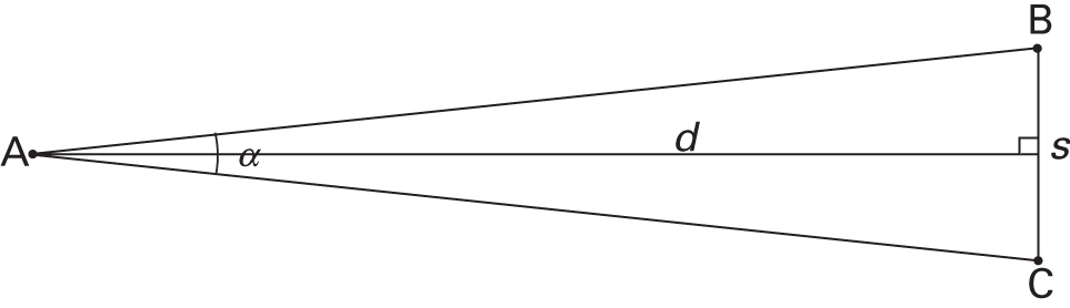
What to notice: Angular size comes from geometry: the same physical size \(s\) subtends a smaller angle \(\\alpha\) at larger distance \(d\). (Credit: Fundamentals of Astrophysics (Owocki))

By definition of angle in radians: \[\alpha (\text{radians}) = \frac{\text{arc length}}{\text{radius}} \approx \frac{s}{d}\]

This is the small-angle approximation:

\[ s = \alpha \, d \tag{1}\]

Small-angle approximation

What it predicts
Given angular size \(\alpha\) (radians) and distance \(d\), it predicts the true physical size \(s\) of an object (or vice versa).

What it depends on
Scales as \(s \propto \alpha d\); angular size is inversely proportional to distance at fixed physical size.

What it's saying
For small angles, the arc length equals the chord length — geometry becomes simple multiplication. Angular size, physical size, and distance form a triangle; know any two, infer the third.

Assumptions

• Angle is small (\(\alpha \lesssim 0.1\) rad \(\approx\) 6°)
• Uses \(\sin\alpha \approx \alpha\) (radians); error is \(<0.5\%\) for \(\alpha < 0.1\) rad
• Both \(s\) and \(d\) must be in the same length units

See: the equation

TipWhat You Should Be Able to Do Now

After reading the small-angle equation, you should be able to:

1. Sketch the triangle that defines \(\alpha\), \(s\), and \(d\)
2. State which unit \(\alpha\) must be in for the formula to work without a conversion factor (radians)
3. Predict: if \(d\) doubles while \(s\) stays fixed, what happens to \(\alpha\)?

NoteEnrichment: Alternative Geometry View

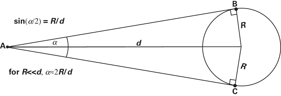
What to notice: The exact relation \(\\sin(\\alpha/2)=R/d\) reduces to \(\\alpha\\approx2R/d\) when \(R\\ll d\), which is the small-angle approximation used in astronomy. (Credit: Fundamentals of Astrophysics (Owocki))

This figure shows the same geometry from a slightly different perspective, reinforcing that the small-angle approximation is just the statement that arc length \(\approx\) chord length for small angles.

Physical meaning: This says that angular size is inversely proportional to distance. A distant object appears small; a nearby object appears large.

ImportantUnits Are Crucial

When you use this formula, be ruthlessly careful about units:

• In radians: \(\alpha_{\text{rad}} \approx s/d\) (both \(s\) and \(d\) in the same units)
• In arcseconds: We must convert from radians to arcseconds using our conversion factor:

\[\alpha_{\text{arcsec}} = \frac{s}{d} \times 206{,}265\]

If \(d\) is in parsecs and \(s\) is measured in AU (or any consistent units), this formula is exact for the parallax angle. This conversion factor is so important that it deserves its own box.

TipQuick Check Yourself

The Moon subtends about \(0.5^\circ\) in our sky. Its distance is approximately \(3.84 \times 10^{10}\) cm. Use the small-angle formula to estimate the Moon’s true diameter.

Hint: First convert \(0.5^\circ\) to arcseconds, then to radians, then apply the formula. Think before checking below.

Note

Convert: \(0.5^{\circ} = 30\) arcmin \(= 1800\) arcsec

In radians: \(1800 \text{ arcsec} \div 206{,}265 \text{ arcsec rad}^{-1} = 0.00873\) rad

True size (diameter): \(s = \alpha \, d = (0.00873 \text{ rad})(3.84 \times 10^{10} \text{ cm}) \approx 3.35 \times 10^{8} \text{ cm} \approx 3{,}350\) km

The actual lunar diameter is about 3,474 km, so our estimate agrees to within about 4% — excellent! This confirms both that the small-angle approximation works beautifully at half-degree scales and that our angular measurements are reliable.

When Does the Approximation Break Down?

The small-angle approximation assumes that \(\sin(\alpha) \approx \alpha\) for small angles. This is excellent as long as \(\alpha \lesssim 0.1\) radian, or roughly 5–6 degrees. For angles larger than this, you must use the exact trigonometric formula.

In astronomy, we rarely deal with angles larger than a degree (except when measuring separation between constellation stars). The vast majority of our work — stellar parallax, galaxy sizes, telescope resolution — happens at arcsecond to degree scales, where the small-angle approximation is superb.

---

Part 4: Parallax — Distance from Baseline Geometry

Now we apply the small-angle formula to the most direct distance-measurement technique in astronomy: parallax. The core idea is simple and has been known for centuries: use a long baseline and measure the angular shift of a nearby object against distant, fixed background objects.

TipPlay First: Parallax Interactive

Before reading the derivation, spend 90 seconds with the interactive demo below. Move the star closer and farther, and watch how the parallax angle changes. Then continue reading — the math will make more sense.

If the demo doesn’t load above, open it in a new tab.

The Parallax Angle

Hold your finger at arm’s length and close one eye, then the other. Your finger appears to shift against the background. The farther away your finger is, the smaller this shift. This is parallax, and it’s the foundation of depth perception in human vision.

The geometry is just the small-angle formula rearranged. Recall the small-angle formula: \(s = \alpha \, d\). In a parallax measurement, we map the variables as follows:

• The “size” \(s\) is the baseline \(b\) — the physical separation between your two viewpoints.
• The “angle” \(\alpha\) is the parallax angle \(p\) — the angular shift you measure.
• The “distance” \(d\) is the distance to the object — the quantity we want to find.

Substituting these into the small-angle formula gives \(b = p \, d\). Solving for \(d\):

\[ d = \frac{b}{p} \tag{2}\]

Parallax-distance relation (general baseline)

What it predicts
Given a baseline length \(b\) and measured parallax angle \(p\) (radians), it predicts the distance \(d\) to the object.

What it depends on
Scales as \(d \propto b\) and \(d \propto p^{-1}\). Longer baselines probe greater distances; smaller parallax angles mean farther objects.

What it's saying
Parallax is the small-angle formula applied to distance measurement. The baseline sets the distance reach — a longer baseline lets you measure smaller angles and therefore greater distances. This equation works for any baseline: the diameter of your head (binocular vision), the radius of Earth's orbit (stellar parallax), or the orbit of Jupiter (if you could observe from there).

Assumptions

• Small-angle regime (\(p \ll 1\) rad)
• Baseline \(b\) is known precisely
• Background reference objects are effectively at infinity

See: the equation

where \(b\) is the baseline length, \(p\) is the parallax angle in radians, and \(d\) is the distance in the same units as \(b\). This is the general parallax-distance relation — it works for any baseline and any observer.

The Baseline Determines the Reach

This is worth pausing on. The distance you can probe is set by the length of your baseline:

• Your head (\(b \approx 7\) cm, the distance between your eyes): you perceive depth out to a few meters — that’s binocular vision.
• Earth’s diameter (\(b \approx 12{,}700\) km): radar ranging to nearby planets, but useless for stars.
• Earth’s orbit (\(b = 1\) AU \(\approx 1.5 \times 10^{13}\) cm): this is what makes stellar parallax possible.
• Jupiter’s orbit (\(b \approx 5.2\) AU): if you could observe from Jupiter, you’d measure parallax angles \(5.2\times\) larger for any star at the same distance — or equivalently, reach \(5.2\times\) farther at the same angular precision.

The physics is always the same (\(d = b/p\)). What changes is the baseline, and therefore the distance reach. Every parallax measurement implicitly encodes a choice of baseline.

Stellar Parallax: Earth’s Orbit as Baseline

In astronomy, Earth’s orbit provides the baseline. As Earth moves from one side of the Sun to the opposite side — a baseline of 2 AU — a nearby star appears to shift against the distant background stars. This shift is parallax.

We define the parallax angle (\(p\)) carefully: it is half the total angular shift, corresponding to a baseline of 1 AU (the orbital radius, not diameter). In other words, \(p\) is the angle subtended by Earth’s orbital radius as seen from the star.

What to notice: A nearby star shifts against distant background stars between January and July; that angular shift is parallax and gives distance. (Credit: cococubed.com)

TipGuided Reading: Study This Figure

Before moving on, identify these elements in the figure above:

1. Point to the baseline. What is its length? (1 AU — Earth’s orbital radius.)
2. Point to \(p\). Where is the parallax angle measured — at Earth or at the star?
3. Think: If \(p\) shrinks by a factor of 2, what happens to \(d\)? (It doubles — \(d = 1/p\).)

This definition is chosen by convention to keep the numbers simple. When you measure a star at opposite sides of Earth’s orbit (six months apart), the total shift is \(2p\); the parallax angle is \(p\). (In reality, the apparent motion of a star over the year traces an ellipse on the sky, not a simple back-and-forth line; \(p\) is defined as the semi-major axis of that ellipse.)

WarningMisconception Alert: Parallax Is Not Angular Size

Parallax and angular size are both measured in arcseconds, but they describe completely different things. Angular size is how big an object looks (e.g., the Moon spans \(0.5^\circ\)). Parallax is how much an object’s position shifts against the background when viewed from two different vantage points. Stars have no measurable angular size — they are unresolved points — yet they have perfectly measurable parallax angles. Do not confuse the two.

WarningMisconception Alert: \(p\) Is Half the Total Shift

A common error is to use the full six-month angular shift as \(p\). Remember: the total back-and-forth shift across six months is \(2p\). The parallax angle \(p\) corresponds to a 1 AU baseline (Earth’s orbital radius), not the full 2 AU diameter. If a problem gives you the total angular shift, divide by 2 before applying \(d = 1/p\).

From General Parallax to the Parsec

Substituting Earth’s baseline \(b = 1\) AU into the general parallax formula:

\[p (\text{radians}) \approx \frac{1 \text{ AU}}{d}\]

Convert to arcseconds: \[p (\text{arcsec}) = \frac{1 \text{ AU}}{d} \times 206{,}265 \text{ arcsec/rad}\]

Rearrange for distance: \[d = \frac{206{,}265 \text{ AU}}{p (\text{arcsec})}\]

This is the fundamental parallax formula for Earth-based observers. But astronomers have made a brilliant choice: define a new distance unit to make this formula even simpler.

The Parsec — A Unit Tied to Earth’s Orbit

Definition: One parsec (pc) is defined as the distance at which a star has a parallax angle of exactly 1 arcsecond when observed from Earth’s orbit (baseline = 1 AU).

From our formula above, if \(p = 1\) arcsec, then: \[1 \text{ pc} = 206{,}265 \text{ AU}\]

This means the distance-parallax relationship becomes breathtakingly simple:

\[ d(\text{pc}) = \frac{1}{p(\text{arcsec})} \tag{3}\]

Parallax-distance relation (Earth baseline, parsec form)

What it predicts
Given stellar parallax \(p\) in arcseconds (measured from Earth's orbit), it predicts the distance \(d\) in parsecs.

What it depends on
Scales as \(d \propto p^{-1}\). Halving the parallax doubles the inferred distance.

What it's saying
This compact form hides two specific choices: (1) baseline = 1 AU (Earth's orbital radius), and (2) angle measured in arcseconds. The parsec is defined as the distance at which 1 AU subtends 1 arcsecond. It is not a universal constant of nature — it is a unit tied to Earth's orbit. An observer on Jupiter (\(b \approx 5.2\) AU) using the same angular units would define a 'Jupiter-parsec' 5.2 times larger.

Assumptions

• Baseline is Earth's orbital radius (1 AU)
• Parallax angle \(p\) is in arcseconds
• Small-angle regime (always satisfied for stellar parallax)
• Background reference stars are effectively at infinity

See: the equation

TipWhat You Should Be Able to Do Now

After reading the parallax-parsec equation, you should be able to:

1. Calculate the distance (in pc) for any star whose parallax is given in arcseconds
2. Explain why this formula only works when \(p\) is in arcseconds and \(b = 1\) AU
3. State the general formula (\(d = b/p\)) and identify which assumption converts it to \(d = 1/p\)

A star with parallax 0.5 arcsecond is at 2 pc. A star with parallax 0.1 arcsecond is at 10 pc. The exact relation is \(\tan p = b/d\), but for stellar parallax \(p\) is so tiny that \(\tan p \approx p\) to absurd precision — the inverse relationship \(d = 1/p\) is effectively exact and extremely convenient.

The name “parsec” comes from parallax arcsecond — it’s not arbitrary. It emerges naturally from choosing 1 AU as the baseline and 1 arcsecond as the angular unit.

NoteEnrichment: Textbook Parallax Geometry

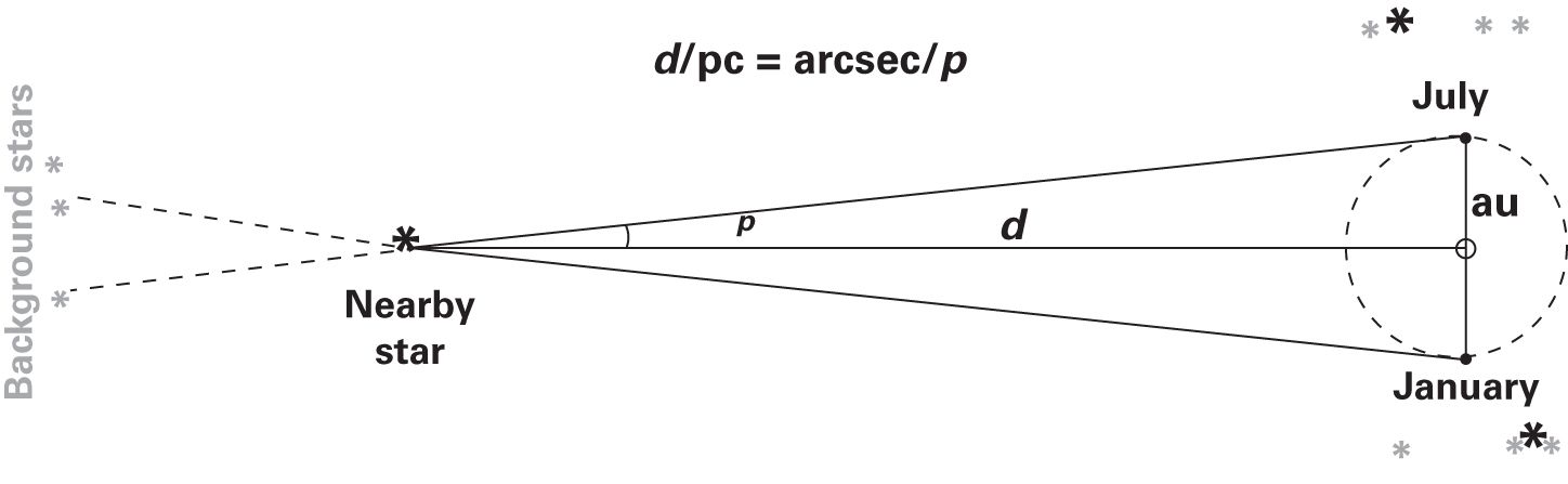
What to notice: Parallax uses Earth’s 1 AU orbital radius as a baseline; the relation \(d(\\text{pc})=1/p(\\text{arcsec})\) turns tiny angles into distances. (Credit: Fundamentals of Astrophysics (Owocki))

This figure from Owocki shows the same stellar parallax geometry from a textbook perspective, reinforcing the relationship between baseline, parallax angle, and distance.

ImportantThe Parsec Is Not a Universal Constant

The parsec is defined relative to Earth’s orbital radius. It is a human unit, not a law of nature. If astronomers lived on Jupiter (\(b \approx 5.2\) AU), the same “parallax of 1 arcsecond” would correspond to a distance of \(5.2 \times 206{,}265\) AU \(\approx 1{,}070{,}000\) AU — about 5.2 pc. A “Jupiter-parsec” would be 5.2 times larger than our parsec.

The compact formula \(d(\text{pc}) = 1/p\) works only because we’ve baked Earth’s baseline into the definition of the parsec. If the baseline changes, the unit changes. Always remember: the general formula \(d = b/p\) is the physics; \(d(\text{pc}) = 1/p(\text{arcsec})\) is a convenient specialization for Earth-bound astronomers.

Convert to more familiar units:

• 1 pc = \(3.09 \times 10^{18}\) cm (approximately \(3 \times 10^{18}\) cm)
• 1 pc = 3.26 light-years
• 1 kiloparsec (kpc) = 1000 pc

TipQuick Check Yourself

Sirius, the brightest star in the night sky, has parallax \(p = 0.379\) arcsecond. How far away is it?

Think first before checking below.

Note

\[d = \frac{1}{0.379 \text{ arcsec}} = 2.64 \text{ pc}\]

Convert to light-years: \(2.64 \text{ pc} \times 3.26 \text{ ly pc}^{-1} = 8.6\) ly

This is correct — Sirius is indeed one of the nearest stars to Earth.

Worked Example: Proxima Centauri

Given: Proxima Centauri, the nearest known star to the Sun (excluding the Sun itself), has a parallax angle \(p = 0.768\) arcsecond.

Find: Distance in parsecs and centimeters.

Step 1: Apply the parallax formula

\[d = \frac{1}{p} = \frac{1}{0.768 \text{ arcsec}} = 1.30 \text{ pc}\]

Step 2: Convert to centimeters

\[d = 1.30 \text{ pc} \times 3.09 \times 10^{18} \text{ cm pc}^{-1} = 4.02 \times 10^{18} \text{ cm}\]

Step 3: Sanity check

Nearby stars should be in the range 1–5 pc. Our answer fits perfectly. ✓

Step 4: Interpret

Proxima Centauri is the nearest known star. At 1.3 pc, it’s about 25 trillion miles away — farther than anything human-made has ever traveled. Yet it’s so close that its parallax was measurable (though barely) from ground-based telescopes, and easily detectable by space missions. This illustrates why parallax measurement was historically so difficult and why measuring it well was so transformative.

NoteExplore: The Solar Neighborhood in 3D

What to notice: The nearest stellar neighborhood is a sparse 3D map around the Sun, with distance rings (3, 6, and 10 light-years) and stars not confined to one plane. (Credit: cococubed.com)

This map shows our nearest stellar neighbors. Notice how Proxima Centauri, at 1.3 pc, is the closest — but many other stars crowd the 2–5 pc range.

NoteEnrichment: From Hipparcos to Gaia — The Parallax Revolution

Pre-1600s: Astronomers looked for parallax but never found it, even for the brightest stars. This wasn’t a technical limitation — it was a fundamental limitation of naked-eye observation. Parallax angles are tiny, and parallax shifts require precise astrometry (position measurement) from year to year. Without telescopes and precise instruments, the shift was invisible against observational noise.

1838: Friedrich Wilhelm Bessel, Thomas Henderson, and Friedrich Georg Wilhelm Struve independently measured parallaxes for nearby stars using telescopes. For the first time, astronomers had direct, geometric proof that stars were at different distances — and that the Sun was not at the center of everything (though this had been accepted on theoretical grounds since Newton). These were the first parallax measurements and a watershed moment in astronomy.

20th century: Ground-based parallax measurements improved gradually, but remained limited to nearby, bright stars. Atmospheric turbulence and instrumental precision restricted the catalog to roughly 1,000 stars with reliable parallaxes.

Hipparcos (1989–1993): The first space-based parallax mission achieved roughly 1 milliarcsecond precision. This extended parallax measurements to about 100,000 stars and out to distances of roughly 100 pc.

Gaia (2013–2025; data releases ongoing): The Gaia astrometry mission represents a genuine revolution. With approximately 10 microarcsecond precision (about \(100\times\) better than Hipparcos), Gaia has measured parallaxes for roughly 1.8 billion stars. The distance reach extends to kiloparsecs, mapping the structure and motion of the entire Milky Way. Gaia completed its science observations in January 2025, but data processing continues — Data Release 4 is expected in late 2026.

NoteExplore: Nearby Massive Stars in 3D

What to notice: Massive stars are rarer and generally farther away than the nearest low-mass stars, so the local sample extends out to several tenths of a kiloparsec. (Credit: cococubed.com)

This map shows the massive stars in our neighborhood. Notice how rare they are compared to the red dwarfs and Sun-like stars shown in the earlier map — massive stars are intrinsically uncommon, but their high luminosity makes them visible at great distances.

ImportantWhy Gaia Changed Everything

Gaia did not just measure more parallaxes — it fundamentally transformed stellar astrophysics. A factor-of-100 improvement in parallax precision directly translates to a \(100\times\) reduction in luminosity uncertainty (as we’ll derive in Part 6). But the impact goes beyond precision for individual stars: Gaia’s reach extends to kiloparsecs, opening up roughly a million times more volume than Hipparcos could survey. This has reshaped our understanding of stellar populations, ages, and evolution across the galaxy. It has also directly enabled the study of exoplanet host stars — something impossible with less precise parallax data.

TipQuick Check Yourself

Estimate the parallax angle for a star at 1 kiloparsec (1000 pc) distance.

Think first before checking below.

Note

\[p = \frac{1}{d} = \frac{1}{1000 \text{ pc}} = 0.001 \text{ arcsec} = 1 \text{ milliarcsecond}\]

This is right at the limit of Hipparcos precision and well within Gaia’s reach.

WarningWhen Does \(d = 1/p\) Break Down?

The simple inversion \(d = 1/p\) works beautifully when \(p\) is measured precisely. But when the uncertainty in \(p\) is comparable to \(p\) itself — or when noise makes the measured parallax negative — simple inversion becomes unreliable or undefined. For such stars, astronomers use more careful statistical inference methods (e.g., Bayesian priors on distance distributions). You won’t need these techniques in this course, but knowing the limitation exists prevents confusion when working with real catalogs.

---

Part 5: The Inverse-Square Law — Two Derivations

We now turn to the second pillar of distance measurement: understanding how light spreads as it travels from a star to Earth. The inverse-square law is one of the most important relationships in physics. It governs not just light, but gravity, electrostatic force, and any phenomenon where something spreads isotropically from a point source.

TipPredict First

Before reading the derivation, try to answer: if you move twice as far from a light source, by what factor does the brightness change? What about 10 times farther? Think about why before reading on.

Geometric Derivation: Concentric Spheres

Imagine a star at the center of a sphere, emitting light uniformly in all directions. The star has a total luminosity \(L\) — the total power (energy per unit time) radiated in all directions.

At a distance \(d\) from the star, this energy is spread over a sphere of surface area:

\[A(d) = 4\pi d^2\]

The flux at distance \(d\) is the energy per unit time per unit area:

\[\boxed{F(d) = \frac{L}{4\pi d^2}}\]

This is the inverse-square law. Let’s understand why it has this form.

The physics: The same total energy \(L\) flows through every spherical shell around the star. At smaller radius, the area is smaller, so the energy is concentrated — flux is high. At larger radius, the area grows as \(d^2\), so the flux spreads out and drops. The \(4\pi\) is the factor that accounts for a full sphere (a solid angle of \(4\pi\) steradians — the total solid angle around a point).

Alternative statement: If you double your distance from a star, the flux drops by a factor of 4. If you go 10 times farther, the flux drops by 100. This \(1/d^2\) relationship is exact for isotropic point sources and no absorption.

ImportantMeaning Card: The Inverse-Square Law

• What it predicts: Given a star’s luminosity and distance, calculate the flux you observe
• What it depends on: Star’s total luminosity (\(L\)), distance (\(d\))
• Key assumption: Isotropic emission (no beaming in any direction), no absorption between star and observer
• Units check: Flux has dimensions of power per area; \(L\) is power; dividing by area gives the right dimensions

These assumptions are sometimes violated. Dust between the star and observer absorbs light (extinction). Some sources (like pulsars) beam radiation preferentially in one direction. Real measurements require correcting for these complications.

NoteExplore: What Happens When Dust Absorbs Light?

Suppose interstellar dust absorbs half the light from a star before it reaches your detector. You measure a flux \(F_{\text{obs}} = F_{\text{true}}/2\). If you naively apply the standard candle formula without correcting for dust:

\[d_{\text{naive}} = \sqrt{\frac{L}{4\pi F_{\text{obs}}}} = \sqrt{\frac{L}{4\pi (F_{\text{true}}/2)}} = \sqrt{2}\;\sqrt{\frac{L}{4\pi F_{\text{true}}}} = \sqrt{2}\;d_{\text{true}}\]

You would overestimate the distance by a factor of \(\sqrt{2} \approx 1.41\) — about 41% too far. This is why dust corrections (called extinction corrections) are essential. Astronomers measure reddening — the wavelength-dependent dimming caused by dust — and remove it before computing distances and luminosities.

Dimensional Analysis Derivation

Here’s a second path to the same result, using dimensional analysis. This approach is faster and requires no geometric picture — only logic about dimensions.

We want to relate three quantities: flux \(F\), luminosity \(L\), and distance \(d\). Assume flux scales as a power law:

\[F \propto L^a d^b\]

Now examine the dimensions of each quantity using the mass-length-time system \([M L T^{-3}]\):

Quantity	Dimension
\(F\) (flux)	\([M L^0 T^{-3}]\) (power per area)
\(L\) (luminosity)	\([M L^2 T^{-3}]\) (power)
\(d\) (distance)	\([L]\)

For the dimensions to match on both sides:

\[[M L^0 T^{-3}] = [M L^2 T^{-3}]^a [L]^b = [M^a L^{2a+b} T^{-3a}]\]

Matching exponents:

• Mass: \(1 = a \Rightarrow a = 1\)
• Time: \(-3 = -3a\) ✓ (consistent with \(a = 1\))
• Length: \(0 = 2a + b = 2(1) + b \Rightarrow b = -2\)

So \(F \propto L^1 d^{-2}\), or:

\[F \propto \frac{L}{d^2}\]

The proportionality constant is \(1/(4\pi)\), which dimensional analysis alone cannot determine — it comes from geometry (the full solid angle of a sphere). But the \(L/d^2\) scaling is certain:

\[\boxed{F = \frac{L}{4\pi d^2}}\]

ImportantWhy Both Derivations?

These two completely different approaches — geometry and dimensional analysis — give the same answer. This convergence should give you confidence. Geometry gives intuition and the \(4\pi\) factor. Dimensional analysis is faster and works even when geometry isn’t obvious. Together, they show that the \(1/d^2\) scaling is not a coincidence; it’s a consequence of how space works.

WarningMisconception Alert: Flux vs. Luminosity

Flux is what your detector measures — it depends on where you stand. Luminosity is what the star emits — it’s an intrinsic property that doesn’t change with the observer’s distance. A dim red dwarf nearby can have the same observed flux as a luminous giant far away. You cannot determine luminosity from flux alone; you always need distance.

TipArgue With a Peer

Two stars have exactly the same apparent brightness in your telescope. Your lab partner says they must have the same luminosity. Do you agree or disagree? Write a one-sentence rebuttal or defense before reading on.

The Flux-Luminosity-Distance Equation

\[ F = \frac{L}{4\pi d^2} \tag{4}\]

Inverse-square relation (flux, luminosity, distance)

What it predicts
Given \(L\) and \(d\), it predicts the observed flux \(F\) at the detector.

What it depends on
Scales as \(F \propto L\) and \(F \propto d^{-2}\).

What it's saying
Apparent brightness mixes intrinsic power and distance; to infer \(L\) from \(F\), you must also know \(d\).

Assumptions

• Approximately isotropic emission (radiates equally in all directions)
• Negligible absorption/scattering between source and observer

See: the equation

TipWhat You Should Be Able to Do Now

After reading the flux-luminosity-distance equation, you should be able to:

1. Rearrange \(F = L/(4\pi d^2)\) to solve for \(L\) or \(d\)
2. Predict by what factor the flux changes if the distance triples
3. Explain why you need both flux and distance to determine luminosity

This equation is the cornerstone of all stellar luminosity measurements. Let’s parse its meaning:

• Observable: Flux \(F\) is measured from photometry (how bright the star appears)
• Model: The inverse-square law (assumption: isotropic emission, no absorption)
• Inference: If we know \(d\) (from parallax), we can rearrange to solve for \(L\)

The equation can be rearranged into three useful forms:

1. Given luminosity and distance, find flux: \(F = L/(4\pi d^2)\)
2. Given flux and distance, find luminosity: \(L = 4\pi d^2 F\)
3. Given luminosity and flux, find distance: \(d = \sqrt{L/(4\pi F)}\)

Form (2) is what we use to build the HR diagram. Form (3) is what we use for standard candles (next section).

---

Part 6: From Distance to Luminosity

Now we bring together parallax and the inverse-square law. This is where the real power of stellar astrophysics emerges: measured distance plus measured brightness gives intrinsic luminosity.

The Measurement Chain

Here is the complete Observable \(\to\) Model \(\to\) Inference sequence for inferring stellar luminosity:

1. Observable 1: Measure the star’s position on the sky repeatedly over months. The position shifts slightly because Earth orbits.
2. Model 1: Apply parallax geometry to convert the angular shift into distance.
3. Observable 2: Measure the star’s brightness in multiple photometric filters to estimate its total (bolometric) flux across all wavelengths. (In practice, bolometric flux is estimated from multi-filter photometry combined with atmospheric models; we’ll return to bolometric corrections in Module 2, Lecture 5.)
4. Model 2: Apply the inverse-square law.
5. Inference: Combine: \(L = 4\pi d^2 F\).

Each step makes assumptions. The parallax model assumes Earth’s orbit is known (it is, to exquisite precision). The flux model assumes isotropic emission and no absorption (nearly true, though dust can absorb starlight). Understanding what can fail — and how to check — is essential.

TipWorked Example: The Solar Constant and Solar Luminosity

Given: - Solar constant (flux from Sun at Earth): \(F_{\odot} = 1.4 \times 10^{6}\) erg cm\(^{-2}\) s\(^{-1}\) - Earth-Sun distance: \(d = 1\) AU = \(1.5 \times 10^{13}\) cm

Find: Solar luminosity \(L_{\odot}\)

Step 1: Rearrange the flux-luminosity-distance equation

\[L = 4\pi d^2 F\]

Step 2: Substitute values

\[L_{\odot} = 4\pi \, (1.5 \times 10^{13} \text{ cm})^2 \times (1.4 \times 10^{6} \text{ erg cm}^{-2}\text{ s}^{-1})\]

\[= 4\pi \times (2.25 \times 10^{26} \text{ cm}^2) \times (1.4 \times 10^{6} \text{ erg cm}^{-2}\text{ s}^{-1})\]

\[= 4\pi \times 3.15 \times 10^{32} \text{ erg s}^{-1}\]

\[= 12.56 \times 3.15 \times 10^{32} \text{ erg s}^{-1}\]

\[\approx 3.96 \times 10^{33} \text{ erg s}^{-1}\]

Step 3: Compare to standard value

The accepted solar luminosity is \(L_{\odot} = 3.828 \times 10^{33}\) erg s\(^{-1}\). Our calculation agrees to within 4% — excellent agreement. Notice how the cm\(^2\) in the distance squared cancels the cm\(^{-2}\) in the flux, leaving us with pure erg s\(^{-1}\) (power) — exactly as expected for luminosity.

What this shows: This is not an alternative way to measure the Sun’s luminosity; this is how we know it. We measure the solar constant at Earth’s orbit (by satellite), measure Earth’s distance from the Sun (by radar and orbital dynamics), and use the inverse-square law. Every star on the HR diagram was placed there using this identical method: measure flux, measure distance, calculate luminosity.

Error Propagation: Why Precision Matters

TipPredict First

Suppose Gaia improves parallax precision by a factor of 100 compared to Hipparcos (from \(\sim 1\) milliarcsecond to \(\sim 10\) microarcseconds). How much does the luminosity uncertainty improve — by the same factor of 100, more, or less? Make a prediction and reason about why, then read on.

Here’s a critical insight. If your parallax measurement has uncertainty, how does that affect your luminosity inference?

Step 1: Parallax \(\to\) Distance. Since \(d = 1/p\), the fractional uncertainty propagates directly: \(\delta d / d = \delta p / p\) (to first order). A 10% parallax uncertainty gives roughly a 10% distance uncertainty. You can verify this: if \(p\) is uncertain by a factor of 1.1, then \(d = 1/(1.1\,p) \approx 0.91\,d\) — about a 9% shift, consistent with the first-order estimate.

Step 2: Distance \(\to\) Luminosity. Since \(L = 4\pi d^2 F\) and distance appears squared, the fractional uncertainty doubles: \(\delta L / L \approx 2 \, (\delta d / d)\). A 10% distance error becomes roughly a 20% luminosity error.

The complete chain: 10% parallax uncertainty \(\to\) ${}$10% distance uncertainty \(\to\) ${}$20% luminosity uncertainty. Errors in parallax cascade through to luminosity with this amplification. This is why improving parallax precision is so valuable — Gaia’s \(100\times\) improvement in parallax precision translates directly to a \(100\times\) improvement in luminosity precision for any given star.

TipQuick Check Yourself

A star has parallax \(p = 0.1\) arcsec and observed flux \(F = 10^{-11}\) erg cm\(^{-2}\) s\(^{-1}\).

1. What is its distance in parsecs and centimeters?

2. What is its luminosity in solar luminosities?

Think first before checking below.

Note

(a) Distance: \[d = \frac{1}{0.1 \text{ arcsec}} = 10 \text{ pc} = 10 \text{ pc} \times 3.09 \times 10^{18} \text{ cm pc}^{-1} = 3.09 \times 10^{19} \text{ cm}\]

(b) Luminosity: \[L = 4\pi d^2 F = 4\pi \,(3.09 \times 10^{19} \text{ cm})^2 \times (10^{-11} \text{ erg cm}^{-2}\text{ s}^{-1})\] \[= 4\pi \times (9.55 \times 10^{38} \text{ cm}^2) \times (10^{-11} \text{ erg cm}^{-2}\text{ s}^{-1})\] \[= 4\pi \times 9.55 \times 10^{27} \text{ erg s}^{-1}\] \[\approx 1.2 \times 10^{29} \text{ erg s}^{-1}\]

Express as solar luminosity: \(L_{\odot} = 3.8 \times 10^{33}\) erg s\(^{-1}\)

\[\frac{L}{L_{\odot}} = \frac{1.2 \times 10^{29} \text{ erg s}^{-1}}{3.8 \times 10^{33} \text{ erg s}^{-1}} \approx 3.2 \times 10^{-5}\]

This is a very faint star — roughly 30,000 times dimmer than the Sun. This is typical for red dwarfs, the most common stars in the galaxy.

Distance Is the Master Key

Here is the big picture. Every other stellar property ultimately depends on distance:

\[\text{Parallax} \xrightarrow{p = 1/d} \text{Distance} \xrightarrow{d \text{ + } F} \text{Luminosity} \xrightarrow{L \text{ + } T} \text{HR Diagram}\]

Once you have distance, the chain unfolds:

• Distance + apparent brightness = luminosity (this lecture)
• Luminosity + effective temperature = stellar radius (Module 2, Lecture 2, via Stefan–Boltzmann: \(L = 4\pi R^2 \sigma T^4\))
• Distance + spectrum = stellar composition (Module 2, Lecture 3)
• Distance + radial velocity of binary = stellar mass (Module 2, Lecture 4)

Each link in the chain amplifies errors. A 1% parallax error becomes \(\sim 1\)% in distance and \(\sim 2\)% in luminosity (because \(L \propto d^2\)), cascading upward through every derived quantity. This is why precision parallax from Gaia has been so revolutionary — it pulls the entire chain taut and makes everything downstream more reliable.

TipWorked Example: The Full Measurement Chain — From Parallax to Astrophysics

Let’s walk through the complete pipeline for a single star to see how parallax, photometry, and the inverse-square law combine to reveal what kind of star we’re looking at.

Given (from Gaia and ground-based photometry):

• Parallax: \(p = 0.214\) arcsec
• Measured flux: \(F = 1.1 \times 10^{-7}\) erg cm\(^{-2}\) s\(^{-1}\)

Step 1: Parallax \(\to\) Distance

\[d = \frac{1}{p} = \frac{1}{0.214 \text{ arcsec}} = 4.67 \text{ pc}\]

Convert: \(d = 4.67 \text{ pc} \times 3.09 \times 10^{18} \text{ cm pc}^{-1} = 1.44 \times 10^{19}\) cm

Step 2: Distance + Flux \(\to\) Luminosity

\[L = 4\pi d^2 F = 4\pi \,(1.44 \times 10^{19} \text{ cm})^2 \times (1.1 \times 10^{-7} \text{ erg cm}^{-2}\text{ s}^{-1})\] \[= 4\pi \times (2.07 \times 10^{38} \text{ cm}^2) \times (1.1 \times 10^{-7} \text{ erg cm}^{-2}\text{ s}^{-1})\] \[= 4\pi \times 2.28 \times 10^{31} \text{ erg s}^{-1} \approx 2.9 \times 10^{32} \text{ erg s}^{-1}\]

Step 3: Compare to the Sun

\[\frac{L}{L_\odot} = \frac{2.9 \times 10^{32} \text{ erg s}^{-1}}{3.83 \times 10^{33} \text{ erg s}^{-1}} \approx 0.075\]

Step 4: Interpret — what kind of star is this?

This star is about 13 times dimmer than the Sun. At 4.67 pc it’s one of our nearest neighbors. A luminosity of \(\sim 0.08\,L_\odot\) is characteristic of a late K or early M dwarf — a small, cool, red star. This is exactly the kind of star that dominates the lower main sequence of the HR diagram, and it illustrates the full power of the measurement chain: a tiny angular shift in the sky, combined with a brightness measurement, reveals the fundamental nature of a star.

TipPredict First

Which would appear brighter in our sky: a faint red dwarf at 2 pc, or a luminous blue giant at 500 pc? Could they ever look identical? Think about what determines apparent brightness before moving on to standard candles.

---

Part 7: Standard Candles — A Preview

We’ve seen how parallax + inverse-square law determines distance. But parallax only works out to about 100 pc with ground-based telescopes, and perhaps 10 kpc with Gaia — far too close to see most of the Milky Way or any other galaxy.

How do astronomers measure distances beyond parallax? By inverting the relationship one more time.

Using the Inverse-Square Law Backwards

If we know the intrinsic luminosity of a star (from theory, calibration, or physical principles), we can measure its flux and infer its distance:

\[d = \sqrt{\frac{L}{4\pi F}}\]

Objects whose intrinsic luminosity is known or determinable are called standard candles. They are one of the most powerful tools in astronomy for mapping the universe.

TipWorked Example: Standard Candle Distance

Given: A Cepheid variable star has a known luminosity \(L = 10{,}000\,L_\odot = 3.8 \times 10^{37}\) erg s\(^{-1}\) (from its pulsation period). You measure its flux as \(F = 1.0 \times 10^{-14}\) erg cm\(^{-2}\) s\(^{-1}\).

Find: Distance to the Cepheid.

Step 1: Apply the standard candle formula: \[d = \sqrt{\frac{L}{4\pi F}} = \sqrt{\frac{3.8 \times 10^{37} \text{ erg s}^{-1}}{4\pi \times 1.0 \times 10^{-14} \text{ erg cm}^{-2}\text{ s}^{-1}}}\]

Step 2: Evaluate: \[d = \sqrt{\frac{3.8 \times 10^{37}}{1.26 \times 10^{-13}} \text{ cm}^2} = \sqrt{3.0 \times 10^{50} \text{ cm}^2} \approx 1.7 \times 10^{25} \text{ cm}\]

Step 3: Convert to parsecs: \[d = \frac{1.7 \times 10^{25} \text{ cm}}{3.09 \times 10^{18} \text{ cm pc}^{-1}} \approx 5.5 \times 10^{6} \text{ pc} = 5.5 \text{ Mpc}\]

Interpret: This Cepheid is about 5.5 Mpc away — well beyond the Milky Way, placing it in a nearby galaxy. This is far beyond parallax reach, illustrating why standard candles are essential for extragalactic distance measurements.

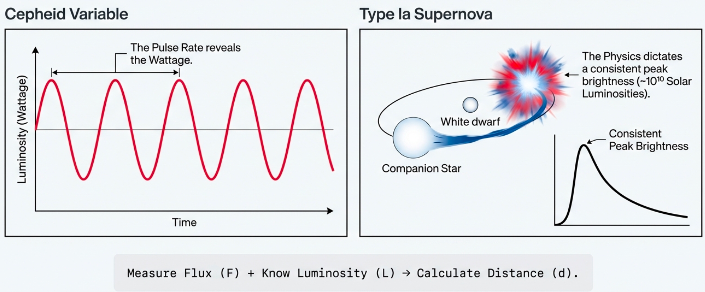
What to notice: Standard candles work because physics predicts their luminosity. Measure flux (F) + know luminosity (L) → calculate distance (d). (Credit: Course illustration (A. Rosen))

Cepheid Variables

Cepheids are pulsating stars that regularly brighten and dim over days to months. In 1912, Henrietta Leavitt discovered something remarkable: the period of pulsation is directly related to intrinsic luminosity. A Cepheid that pulsates once per week is intrinsically brighter than one that pulsates once per day.

This period-luminosity relation is a physical consequence of stellar structure — essentially, a larger (more luminous) star oscillates more slowly. The important point for us: if you measure a Cepheid’s period, you immediately know its luminosity. Measure its apparent brightness and you get distance.

Cepheids are bright enough to be detected in nearby galaxies. In the 1920s, Edwin Hubble used Cepheids in Andromeda to prove that Andromeda was a separate galaxy far beyond the Milky Way. This single application of distance measurement — the period-luminosity relation applied to Cepheids — reshaped our understanding of the universe’s scale.

Type Ia Supernovae

Type Ia supernovae are thermonuclear explosions of white dwarfs in binary systems. They’re violent, short-lived events. But remarkably, they have roughly similar peak luminosities — a few \(\times 10^9 L_{\odot}\). This makes them excellent standard candles for cosmological distances.

In 1998, observations of Type Ia supernovae in distant galaxies revealed something unexpected: the universe’s expansion is accelerating, not slowing down. This discovery of dark energy won the 2011 Nobel Prize in Physics (awarded to Perlmutter, Schmidt, and Riess). It came directly from using Type Ia supernovae as standard candles to measure distances out to several gigaparsecs.

The Cosmic Distance Ladder

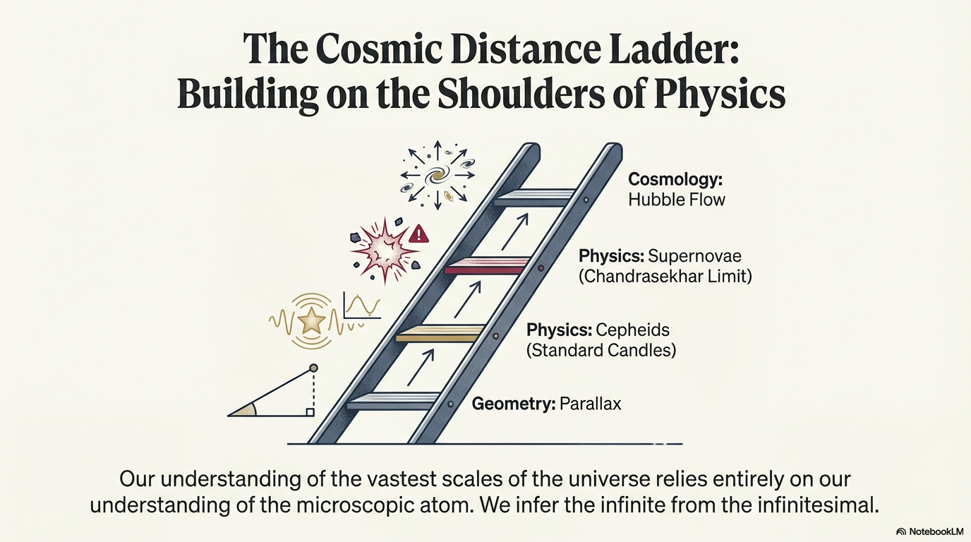
What to notice: Each rung calibrates the next. Parallax (geometry) → Cepheids (standard candles) → Supernovae (Chandrasekhar limit) → Hubble Flow (cosmology). We infer the infinite from the infinitesimal. (Credit: Course illustration (A. Rosen))

The distance ladder links different measurement techniques:

1. Parallax (direct geometry): out to \(\sim 100\) pc from ground, \(\sim 10\) kpc with Gaia
2. Nearby Cepheids (calibrated with parallax): out to \(\sim 30\) Mpc (well beyond the Local Group, which spans \(\sim 3\) Mpc)
3. Type Ia supernovae (calibrated with Cepheids): out to \(\sim 10\) Gpc (edge of observable universe)

Each rung is calibrated using the rung below. The entire cosmic distance scale rests on getting nearby distances right — which is why parallax is so fundamental.

ImportantWhy Getting Nearby Distances Right Matters

When Gaia improved nearby parallaxes by factors of 10–100, it rippled through the entire cosmic distance ladder. Cepheid calibrations became more precise. Type Ia supernova distances became more reliable. Estimates of the universe’s age and composition changed. A seemingly local measurement — parallax for nearby stars — affects our understanding of the entire cosmos. This is why space missions dedicated to parallax measurement (Hipparcos, Gaia) are foundational investments in astronomy.

---

Summary: Observable \(\to\) Model \(\to\) Inference

Here is the complete framework for distance and luminosity measurement:

Measurement Goal	Observable	Model	Inference
Distance	Star’s position shift across sky (arcsec)	Parallax formula: \(d = 1/p\) in pc and arcsec	Distance in parsecs and cm
Distance (alternative)	Angular separation; known baseline (Earth’s orbit = 1 AU)	Small-angle geometry	Same as above
Luminosity	Measured flux from photometry (erg cm\(^{-2}\) s\(^{-1}\))	Inverse-square law: \(F = L/(4\pi d^2)\)	Rearrange to \(L = 4\pi d^2 F\)
Distance (reversed)	Flux; known intrinsic luminosity (e.g., Cepheid period)	Standard candle relation	Use \(d = \sqrt{L/(4\pi F)}\)

Each step has assumptions. Parallax assumes Earth’s orbit is known. The inverse-square law assumes isotropic emission and no absorption. Standard candles assume the calibration is correct. Good science means always asking: what could go wrong?

---

Self-Assessment Checklist

By the end of this lecture, you should be able to check off each of these items. If not, revisit the relevant section.

Angular Measure and Conversion

• I can convert between degrees, arcminutes, and arcseconds fluently
• I understand that radians are dimensionless (a ratio of lengths)
• I can convert between arcseconds and radians using the 206,265 factor
• I know why stellar parallaxes are measured in arcseconds (not radians or degrees)

Small-Angle Approximation

• I can derive \(\alpha \approx s/d\) from a simple geometric triangle
• I understand why the approximation breaks down for large angles (\(> 0.1\) radian)
• I can apply the formula to estimate true sizes or distances of objects
• I understand the conversion between radians and arcseconds when using the formula

Parallax and the Parsec

• I can define the parallax angle \(p\) and explain why it’s measured from the star
• I can derive the relationship \(d(\text{pc}) = 1/p(\text{arcsec})\) using the small-angle formula
• I understand why the parsec is the natural distance unit for parallax measurements
• I can calculate stellar distances from parallax angles
• I know the key conversions: 1 pc = 3.26 light-years = \(3.09 \times 10^{18}\) cm

Parallax Measurement History and Modern Surveys

• I understand why parallax was historically difficult to measure
• I know the precision improvements: Hipparcos (\(\sim 1\) milliarcsecond) to Gaia (\(\sim 10\) microarcseconds)
• I can estimate the distance reach for each mission
• I understand why Gaia’s improved precision transformed all of stellar astrophysics

The Inverse-Square Law

• I can derive the inverse-square law using concentric spheres (geometric approach)
• I can derive it using dimensional analysis
• I understand why both approaches give \(F = L/(4\pi d^2)\)
• I can explain the physical meaning of the \(4\pi\) (full solid angle of a sphere)
• I understand that extinction (dust absorption) breaks this ideal relationship

Flux, Luminosity, and Distance

• I can rearrange \(F = L/(4\pi d^2)\) to solve for \(L\) or \(d\)
• I can apply \(L = 4\pi d^2 F\) to infer stellar luminosity from parallax and photometry
• I understand error propagation: parallax error \(\to\) distance error \(\to\) luminosity error
• I can work through a complete calculation (solar constant example)

Observable \(\to\) Model \(\to\) Inference Framework

• I can identify observables (position shift, brightness)
• I can state the models (parallax geometry, inverse-square spreading)
• I can explain the inferences (distance, luminosity)
• I recognize that each link in the chain makes assumptions

Standard Candles (Preview)

• I understand the concept of a standard candle
• I know that Cepheid variables and Type Ia supernovae serve as distance indicators
• I can apply \(d = \sqrt{L/(4\pi F)}\) if the intrinsic luminosity is known
• I understand the cosmic distance ladder (parallax \(\to\) Cepheids \(\to\) Type Ia supernovae)

---

Practice Problems

Conceptual Problems

1. Why Is Distance Measurement Hard?

Explain why parallax angles for stars are so tiny. Use the small-angle formula to estimate the parallax angle of a star at 100 light-years distance (about 30 pc).

1. Show that \(p \approx 1/d\) (in parsecs and arcseconds), so a star at 30 pc has \(p \approx 0.03\) arcsec.

2. Convert 0.03 arcsec to microarcseconds and compare to Gaia’s precision (\(\sim 10\) \(\mu\)arcsec).

3. Explain why measuring such tiny angles requires space telescopes (ground-based telescopes suffer from atmospheric distortion).

2. Inverse-Square Law and Stellar Brightness

Two identical stars have the same intrinsic luminosity \(L\). Star A is twice as far from Earth as Star B.

1. By what factor is Star A fainter (in observed flux) than Star B?

2. If Star B is observed to have flux \(F_B\), what is the flux of Star A?

3. Conceptual challenge: Explain why the inverse-square law is “universal” — it applies to any kind of radiation (light, radio, X-rays) spreading isotropically from any source.

Calculation Problems

3. Parallax-Distance Conversion

Convert each of the following parallax angles to distances in parsecs, then to light-years:

1. Sirius: \(p = 0.379\) arcsec

2. Vega: \(p = 0.129\) arcsec

3. Altair: \(p = 0.198\) arcsec

4. Computing Stellar Luminosity

A star has parallax \(p = 0.050\) arcsec and observed flux \(F = 5 \times 10^{-13}\) erg cm\(^{-2}\) s\(^{-1}\).

1. Calculate its distance in parsecs and centimeters.

2. Use \(L = 4\pi d^2 F\) to compute the star’s luminosity in erg/s.

3. Express the luminosity as a fraction of the solar luminosity (\(L_{\odot} = 3.8 \times 10^{33}\) erg/s).

4. Sanity check: Is this answer reasonable for a typical star? (Hint: Most stars are dimmer than the Sun.)

5. Error Propagation from Parallax to Luminosity

Gaia measures a star’s parallax as \(p = 0.100 \pm 0.001\) arcsec (1% uncertainty).

1. Calculate the distance: \(d = 10.0 \pm ?\) pc. What is the fractional uncertainty in distance?

2. A photometric measurement gives flux \(F = 1.0 \times 10^{-11} \pm 0.05 \times 10^{-11}\) erg cm\(^{-2}\) s\(^{-1}\) (5% uncertainty).

3. Compute luminosity \(L = 4\pi d^2 F\). What is the fractional uncertainty in luminosity coming from parallax alone?

4. Combined with the 5% photometry uncertainty, what is the total fractional uncertainty in \(L\)?

5. Conclusion: Why is precise parallax so critical for accurate luminosity measurements?

Synthesis Problems

6. The Cosmic Distance Ladder — Parallax vs. Standard Candles

1. Hipparcos (1990): 1 milliarcsecond precision. What is the maximum reliable distance for a star with parallax of (i) 1 arcsec? (ii) 0.001 arcsec?

2. Gaia DR2 (2018): 10 microarcsecond precision. Redo part (a) for Gaia.

3. Gaia future (2030+): 1 microarcsecond precision. Redo part (a).

4. Cepheid variables: A Cepheid in the Andromeda galaxy (distance \(\sim 2.5\) million light-years \(= \sim 770\) kpc) has measured flux \(F = 10^{-14}\) erg cm\(^{-2}\) s\(^{-1}\) and known (from period-luminosity relation) luminosity \(L = 10{,}000 L_{\odot} \approx 3.8 \times 10^{37}\) erg/s.

5. Use the inverse-square law to verify whether the flux and luminosity are consistent at 770 kpc.

2. Why can’t we measure Andromeda’s distance using parallax (even with Gaia)?

3. Explain how the cosmic distance ladder combines parallax (nearby distances) with standard candles (distant distances).

7. From Parallax and Photometry to the HR Diagram

A catalog contains three stars with the following parallaxes and apparent magnitudes (smaller magnitude = brighter):

Star	Parallax (arcsec)	Apparent magnitude
A	0.10	5.0
B	0.010	5.0
C	0.010	3.0

1. Rank the three stars by distance (nearest to farthest).

2. Rank by intrinsic luminosity (brightest to dimmest). Explain your reasoning.

3. Conceptual: Why is it impossible to determine intrinsic luminosity from apparent brightness alone? What information is missing?

4. Write out the complete Observable \(\to\) Model \(\to\) Inference sequence for constructing the HR diagram using parallax and photometry.

---

Glossary & Key Terms

Angular size (angular diameter): The apparent size of an object as seen from Earth, measured in degrees, arcminutes, or arcseconds.

Arcsecond (arcsec): 1/3600 of a degree, or 1/60 of an arcminute; the standard unit for stellar parallax measurements.

Flux: Energy per unit time per unit area (erg cm\(^{-2}\) s\(^{-1}\) in CGS units). Flux decreases with distance as \(1/d^2\).

Hertzsprung-Russell diagram (HR diagram): A plot of stellar luminosity (vertical axis, logarithmic) vs. effective temperature (horizontal axis), revealing stellar properties and evolutionary states.

Inverse-square law: The principle that flux (or gravitational force, electrostatic force) decreases as \(1/d^2\) when spreading isotropically from a point source.

Luminosity: The total power radiated by a star in all directions (erg/s in CGS units). Luminosity is intrinsic — it does not depend on the observer’s distance.

Parallax angle (\(p\)): The apparent angular shift of a nearby star as Earth orbits the Sun, measured from the star (half of the total shift). Units: arcseconds.

Parsec (pc): The distance at which a star has parallax angle \(p = 1\) arcsecond. Equal to \(3.09 \times 10^{18}\) cm, or 3.26 light-years. The natural unit for stellar parallax measurements.

Radian: The natural unit for angles in physics, defined as the angle subtended by an arc whose length equals the radius. \(1 \text{ radian} = 206{,}265 \text{ arcsec}\).

Small-angle approximation: For small angles \(\alpha \ll 1\) radian, \(\sin(\alpha) \approx \tan(\alpha) \approx \alpha\). This simplifies trigonometry and allows direct geometric relationships between angular size, true size, and distance.

Standard candle: An object (Cepheid variable, Type Ia supernova) with known or determinable intrinsic luminosity, allowing distance inference from measured flux using the inverse-square law.

---

Looking Ahead

This lecture has given you the tools to measure distance and infer luminosity. But the HR diagram has two axes — luminosity and temperature. In the next lecture, we’ll apply thermal physics (Stefan-Boltzmann law, Wien’s displacement law) to measure stellar effective temperatures and radii. Together, distance and temperature unlock the HR diagram.

Lecture 2 (next): Surface Flux & Colors of Stars - Apply Stefan-Boltzmann law to relate luminosity and radius to temperature - Use Wien’s law to infer temperature from spectral color - Derive stellar radii from luminosity and temperature

Lecture 3: Spectra & Composition - Identify elements via spectral lines - Classify stars by spectral type (OBAFGKM sequence) - Measure radial velocities with the Doppler effect

Lecture 4: Masses from Motion - Use binary star orbits and Kepler’s third law to measure stellar masses - Establish the mass-luminosity relation

Lecture 5: Magnitudes & the Distance Modulus - Logarithmic brightness scales and the magnitude system - Extend distance measurements beyond parallax with standard candles - Connect apparent magnitude and distance

Lecture 6: Building the HR Diagram - Synthesize all Module 2 tools to plot and interpret the HR diagram - Identify main sequence, giants, white dwarfs - Begin discussing stellar evolution